Comparing two Excel sheets effectively involves identifying differences, inconsistencies, and errors to ensure data accuracy and integrity. At COMPARE.EDU.VN, we provide comprehensive solutions to streamline this process, saving you time and improving your data management. By understanding the right tools and techniques, you can efficiently compare Excel files and maintain data quality.
1. What is the Best Way to Compare Two Excel Sheets for Differences?
The best way to compare two Excel sheets for differences involves using built-in Excel features like conditional formatting, formulas, and specialized tools like Microsoft Spreadsheet Compare. Conditional formatting highlights differing cells, while formulas such as =IF(A1=B1,"Match","Mismatch") can identify discrepancies. For more complex comparisons, Microsoft Spreadsheet Compare, available in Office Professional Plus and Microsoft 365 Apps for enterprise, generates detailed reports on the differences found.
1.1 Using Conditional Formatting for Simple Comparisons
Conditional formatting is a quick and easy way to highlight differences in two Excel sheets. Here’s how to use it:
- Select the Range: Select the range of cells you want to compare in the first sheet.
- Open Conditional Formatting: Go to the “Home” tab, click on “Conditional Formatting,” then “New Rule.”
- Create a New Rule: Choose “Use a formula to determine which cells to format.”
- Enter the Formula: Enter a formula that compares the selected cell to the corresponding cell in the other sheet. For example, if you’re comparing Sheet1 to Sheet2, the formula would be
=A1<>Sheet2!A1. - Set the Formatting: Click on “Format,” choose the formatting style you want to use to highlight the differences (e.g., fill color), and click “OK.”
- Apply the Rule: Click “OK” to apply the conditional formatting rule.
This method instantly highlights any cells in the first sheet that do not match the corresponding cells in the second sheet.
1.2 Employing Formulas to Identify Mismatches
Excel formulas provide a more direct way to identify mismatches between two sheets. The IF formula is particularly useful for this purpose.
- Select a Cell: Choose an empty column next to your data in the first sheet.
- Enter the Formula: In the first cell of the empty column, enter the
IFformula to compare the corresponding cells in both sheets. For example,=IF(Sheet1!A1=Sheet2!A1,"Match","Mismatch"). - Apply the Formula: Drag the fill handle (the small square at the bottom-right of the cell) down to apply the formula to the rest of the column.
This method will display “Match” or “Mismatch” in the column, indicating whether the corresponding cells in both sheets are identical.
1.3 Leveraging Microsoft Spreadsheet Compare for Advanced Analysis
For more in-depth comparisons, Microsoft Spreadsheet Compare offers a comprehensive solution. This tool is particularly useful for identifying complex differences like formula changes, macro differences, and formatting discrepancies.
- Open Spreadsheet Compare: Find and open the “Spreadsheet Compare” application. This tool is available in Office Professional Plus 2013, Office Professional Plus 2016, Office Professional Plus 2019, or Microsoft 365 Apps for enterprise.
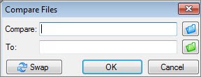
- Compare Files: Click on “Compare Files.”
- Select Files: Choose the two Excel files you want to compare by clicking the blue folder icon next to the “Compare” box and the green folder icon next to the “To” box.
- Choose Options: Select the options you want to include in the comparison, such as “Formulas,” “Macros,” and “Cell Format.”
- Run the Comparison: Click “OK” to run the comparison.
The tool will generate a detailed report highlighting the differences between the two Excel files, making it easier to identify and understand the changes.
2. How Do I Use Excel to Compare Two Columns for Matches and Differences?
To use Excel to compare two columns for matches and differences, employ the IF function along with MATCH or COUNTIF. The IF function displays results based on a condition, while MATCH finds a specific item in a range, and COUNTIF counts cells that meet a criterion. These functions help identify matching and differing entries between columns efficiently.
2.1 Using the IF and MATCH Functions
The IF and MATCH functions can be combined to identify matches and differences between two columns.
- Select a Cell: Choose an empty column next to your data.
- Enter the Formula: In the first cell of the empty column, enter the formula
=IF(ISNUMBER(MATCH(A1,B:B,0)),"Match","Mismatch").A1is the first cell in the first column you want to compare.B:Bis the entire second column.MATCH(A1,B:B,0)searches for the value ofA1in column B and returns its position. If the value is not found, it returns an error.ISNUMBERchecks if the result ofMATCHis a number (i.e., the value was found).IFthen displays “Match” if the value is found and “Mismatch” if not.
- Apply the Formula: Drag the fill handle down to apply the formula to the rest of the column.
This method will display “Match” or “Mismatch” in the column, indicating whether each value in the first column is found in the second column.
2.2 Utilizing the IF and COUNTIF Functions
The IF and COUNTIF functions offer another way to compare two columns.
- Select a Cell: Choose an empty column next to your data.
- Enter the Formula: In the first cell of the empty column, enter the formula
=IF(COUNTIF(B:B,A1)>0,"Match","Mismatch").A1is the first cell in the first column you want to compare.B:Bis the entire second column.COUNTIF(B:B,A1)counts how many times the value ofA1appears in column B.IFthen displays “Match” if the count is greater than 0 (i.e., the value is found) and “Mismatch” if not.
- Apply the Formula: Drag the fill handle down to apply the formula to the rest of the column.
This method also displays “Match” or “Mismatch,” showing whether each value in the first column is present in the second column.
2.3 Highlighting Differences with Conditional Formatting
Conditional formatting can also be used to highlight differences between two columns.
- Select the First Column: Select the range of cells in the first column you want to compare.
- Open Conditional Formatting: Go to the “Home” tab, click on “Conditional Formatting,” then “New Rule.”
- Create a New Rule: Choose “Use a formula to determine which cells to format.”
- Enter the Formula: Enter a formula that checks if the value in the first column is not found in the second column. For example,
=COUNTIF(B:B,A1)=0. - Set the Formatting: Click on “Format,” choose the formatting style you want to use to highlight the differences, and click “OK.”
- Apply the Rule: Click “OK” to apply the conditional formatting rule.
This method highlights any cells in the first column that do not have a corresponding value in the second column.
3. What Excel Function Can I Use to Compare Data in Two Different Sheets?
Several Excel functions can compare data in two different sheets, including VLOOKUP, INDEX/MATCH, and IF. VLOOKUP searches for a value in one sheet and returns a corresponding value from another. INDEX/MATCH provides a more flexible alternative to VLOOKUP. The IF function checks for specific conditions and returns different results based on whether the condition is true or false.
3.1 Using VLOOKUP to Compare Data
The VLOOKUP function is useful for comparing data based on a common identifier.
- Select a Cell: Choose an empty column next to your data in the first sheet.
- Enter the Formula: In the first cell of the empty column, enter the formula
=VLOOKUP(A1,Sheet2!A:B,2,FALSE).A1is the lookup value (the common identifier) in the first sheet.Sheet2!A:Bis the range in the second sheet where the lookup value and the corresponding data are located.2is the column number in the range that contains the data you want to retrieve.FALSEensures an exact match.
- Apply the Formula: Drag the fill handle down to apply the formula to the rest of the column.
This formula searches for the value in A1 of the first sheet in the first column of Sheet2. If it finds a match, it returns the value from the second column of Sheet2. If no match is found, it returns an error (#N/A).
3.2 Using INDEX/MATCH for Flexible Comparisons
The INDEX and MATCH functions can be combined to provide a more flexible alternative to VLOOKUP.
- Select a Cell: Choose an empty column next to your data in the first sheet.
- Enter the Formula: In the first cell of the empty column, enter the formula
=INDEX(Sheet2!B:B,MATCH(A1,Sheet2!A:A,0)).A1is the lookup value (the common identifier) in the first sheet.Sheet2!B:Bis the column in the second sheet that contains the data you want to retrieve.Sheet2!A:Ais the column in the second sheet that contains the lookup values.MATCH(A1,Sheet2!A:A,0)finds the position of the lookup value in the second sheet.INDEXthen retrieves the value from the specified column at the found position.
- Apply the Formula: Drag the fill handle down to apply the formula to the rest of the column.
This formula searches for the value in A1 of the first sheet in the first column of Sheet2. If it finds a match, it returns the corresponding value from the second column of Sheet2.
3.3 Using the IF Function to Check Conditions
The IF function can be used to check specific conditions between two sheets.
- Select a Cell: Choose an empty column next to your data in the first sheet.
- Enter the Formula: In the first cell of the empty column, enter the formula
=IF(Sheet1!A1=Sheet2!A1,"Match","Mismatch").Sheet1!A1is the first cell in the first sheet you want to compare.Sheet2!A1is the corresponding cell in the second sheet.IFthen displays “Match” if the values are identical and “Mismatch” if not.
- Apply the Formula: Drag the fill handle down to apply the formula to the rest of the column.
This method displays “Match” or “Mismatch,” indicating whether the corresponding cells in both sheets are identical.
4. How Do I Compare Two Excel Files Side by Side?
Comparing two Excel files side by side can be done by opening both files and arranging them in separate windows on your screen or by using Excel’s built-in feature to view two sheets simultaneously. Another approach involves using the “New Window” feature to view the same file in two windows, enabling you to compare different parts of the same file.
4.1 Arranging Excel Files in Separate Windows
The simplest way to compare two Excel files is by arranging them in separate windows.
- Open Both Files: Open both Excel files you want to compare.
- Arrange Windows: Go to the “View” tab and click on “Arrange All.”
- Choose Arrangement: Select the arrangement style you prefer (e.g., “Tiled,” “Horizontal,” or “Vertical”) and click “OK.”
Excel will arrange the opened workbooks side by side, making it easy to view and compare them simultaneously.
4.2 Using Excel’s “New Window” Feature
Excel’s “New Window” feature allows you to view different parts of the same workbook in separate windows.
- Open the File: Open the Excel file you want to compare.
- Create a New Window: Go to the “View” tab and click on “New Window.” This opens another instance of the same workbook.
- Arrange Windows: Go to the “View” tab in either window and click on “Arrange All.”
- Choose Arrangement: Select the arrangement style you prefer and click “OK.”
Now, you can navigate to different sheets or sections in each window, making it easier to compare different parts of the same file.
4.3 Utilizing Third-Party Tools for Side-by-Side Comparison
Several third-party tools are available that offer advanced features for comparing Excel files side by side. These tools often provide additional functionalities like highlighting differences, synchronizing scrolling, and generating detailed comparison reports.
Examples of such tools include:
- Microsoft Spreadsheet Compare: As mentioned earlier, this tool provides a detailed comparison report, highlighting differences in formulas, formatting, and other elements.
- Araxis Excel Compare: This tool allows you to compare Excel files and identify differences with color-coded highlights.
- Synkronizer: This tool helps you compare and merge Excel files, making it easier to update and synchronize your data.
5. Is There a Way to Compare Two Excel Sheets Online for Free?
Yes, several online tools allow you to compare two Excel sheets for free. These tools typically require you to upload your Excel files, and they then highlight the differences between them. While convenient, ensure the tool is reputable to protect your data’s privacy and security.
5.1 Using Google Sheets for Online Comparison
Google Sheets offers a free and accessible way to compare two Excel sheets online.
- Upload Files: Upload both Excel files to your Google Drive.
- Open with Google Sheets: Open both files with Google Sheets.
- Use Comparison Formulas: Use the same comparison formulas mentioned earlier (e.g.,
IF,VLOOKUP,INDEX/MATCH) to identify differences between the sheets.
Google Sheets functions similarly to Excel, allowing you to use formulas and conditional formatting to compare data.
5.2 Exploring Online Comparison Tools
Several websites offer free tools to compare Excel sheets online. These tools typically allow you to upload your files and then highlight the differences.
Examples of such tools include:
- Diffchecker: A versatile tool that can compare text, images, and Excel files.
- Aspose.Cells Comparison: An online tool specifically designed for comparing Excel files.
- GroupDocs Comparison: Another online tool that supports various file formats, including Excel.
When using these tools, ensure you review their privacy policies and security measures to protect your data.
5.3 Considerations for Using Online Tools
While online tools offer convenience, it’s essential to consider the following:
- Data Security: Ensure the tool has robust security measures to protect your data from unauthorized access.
- Privacy Policy: Review the privacy policy to understand how your data is used and stored.
- File Size Limits: Be aware of any file size limits that may apply.
- Functionality: Some free tools may have limited functionality compared to desktop software.
6. How Can I Highlight Differences Between Two Excel Sheets?
Highlighting differences between two Excel sheets can be achieved through conditional formatting, formulas, and the Microsoft Spreadsheet Compare tool. Conditional formatting uses rules to automatically format cells based on their values, while formulas like IF can identify mismatches. Microsoft Spreadsheet Compare generates detailed reports with color-coded highlights.
6.1 Using Conditional Formatting for Highlighting
Conditional formatting is a powerful way to highlight differences in Excel.
- Select the Range: Select the range of cells you want to compare in the first sheet.
- Open Conditional Formatting: Go to the “Home” tab, click on “Conditional Formatting,” then “New Rule.”
- Create a New Rule: Choose “Use a formula to determine which cells to format.”
- Enter the Formula: Enter a formula that compares the selected cell to the corresponding cell in the other sheet. For example,
=A1<>Sheet2!A1. - Set the Formatting: Click on “Format,” choose the formatting style you want to use to highlight the differences (e.g., fill color), and click “OK.”
- Apply the Rule: Click “OK” to apply the conditional formatting rule.
This method instantly highlights any cells in the first sheet that do not match the corresponding cells in the second sheet.
6.2 Applying Formulas to Identify and Highlight
Formulas can be combined with conditional formatting to identify and highlight differences.
- Use Comparison Formulas: Use formulas like
IF,VLOOKUP, orINDEX/MATCHto identify differences between the sheets. - Apply Conditional Formatting: Select the column with the formula results and apply conditional formatting to highlight specific outcomes (e.g., highlight “Mismatch” results).
- Create a New Rule: Choose “Format only cells that contain.”
- Set the Rule: Set the rule to format cells that contain specific text (e.g., “Mismatch”).
- Set the Formatting: Choose the formatting style you want to use to highlight the differences and click “OK.”
This method highlights the cells where the comparison formulas indicate a difference.
6.3 Leveraging Microsoft Spreadsheet Compare
Microsoft Spreadsheet Compare automatically highlights differences between two Excel files.
- Open Spreadsheet Compare: Find and open the “Spreadsheet Compare” application.
- Compare Files: Click on “Compare Files.”
- Select Files: Choose the two Excel files you want to compare.
- Run the Comparison: Click “OK” to run the comparison.
The tool will generate a detailed report with color-coded highlights, making it easy to identify the differences.
7. What Are Some Common Errors When Comparing Excel Sheets?
Common errors when comparing Excel sheets include overlooking hidden rows or columns, ignoring case sensitivity, and failing to account for different data types. Additionally, not considering formula differences or ignoring minor formatting discrepancies can lead to inaccurate comparisons. Always double-check settings and use appropriate tools to mitigate these errors.
7.1 Overlooking Hidden Rows or Columns
Hidden rows or columns can lead to inaccurate comparisons because they are not immediately visible.
- Unhide Rows and Columns: Before comparing, ensure all rows and columns are visible.
- Select All: Press
Ctrl+Ato select the entire sheet. - Unhide: Right-click on any row or column header and select “Unhide.”
This ensures that all data is visible and included in the comparison.
7.2 Ignoring Case Sensitivity
Excel is not case-sensitive by default, but sometimes case differences are important.
- Use Case-Sensitive Formulas: Use formulas that account for case sensitivity, such as
=EXACT(A1,Sheet2!A1). This formula returnsTRUEonly if the values are identical, including the case. - Apply Conditional Formatting: Use conditional formatting to highlight case differences based on the
EXACTformula.
This ensures that case differences are identified and highlighted.
7.3 Failing to Account for Different Data Types
Different data types (e.g., numbers formatted as text) can cause comparison errors.
- Check Data Types: Ensure that the data types in both sheets are consistent.
- Use the VALUE Function: Use the
VALUEfunction to convert text to numbers, if necessary. For example,=VALUE(A1)converts the text in cellA1to a number. - Apply Consistent Formatting: Apply consistent formatting to all cells to avoid data type discrepancies.
This ensures that data types are consistent and do not cause comparison errors.
8. How Do I Synchronize Scrolling in Two Excel Windows?
Synchronizing scrolling in two Excel windows allows you to scroll through both sheets simultaneously, making it easier to compare them. Excel does not have a built-in feature for synchronized scrolling, but you can achieve this using VBA macros or third-party add-ins.
8.1 Using VBA Macros for Synchronized Scrolling
VBA macros can be used to synchronize scrolling in two Excel windows.
- Open VBA Editor: Press
Alt+F11to open the VBA editor. - Insert a Module: In the VBA editor, go to “Insert” and select “Module.”
- Enter the Code: Enter the following VBA code into the module:
Public blnSync As Boolean

Sub EnableSync()
    blnSync = True
End Sub

Sub DisableSync()
    blnSync = False
End Sub

Private Sub Workbook_SheetActivate(ByVal Sh As Object)
    If blnSync Then
        Application.OnTime Now, "SyncScroll"
    End If
End Sub

Sub SyncScroll()
    If blnSync Then
        Application.OnTime Now + TimeValue("0:00:01"), "SyncScroll"
        If ActiveWindow.Type = xlNormal Then
            For Each win In Application.Windows
                If win.Type = xlNormal And win.Caption <> ActiveWindow.Caption Then
                    win.ScrollRow = ActiveWindow.ScrollRow
                    win.ScrollColumn = ActiveWindow.ScrollColumn
                End If
            Next win
        End If
    End If
End Sub- Save the Code: Save the VBA code.
- Run the Macro: To start synchronized scrolling, run the
EnableSyncmacro. To stop it, run theDisableSyncmacro.
This VBA code synchronizes the scrolling in all open Excel windows.
8.2 Using Third-Party Add-ins
Several third-party add-ins provide synchronized scrolling as a built-in feature.
Examples of such add-ins include:
- Kutools for Excel: This add-in offers a variety of tools, including synchronized scrolling.
- ASAP Utilities: This add-in also provides synchronized scrolling and other useful features.
These add-ins can simplify the process of synchronizing scrolling in Excel.
8.3 Alternative Methods for Visual Comparison
If synchronized scrolling is not feasible, consider alternative methods for visual comparison.
- Arrange Windows Side by Side: Arrange the Excel windows side by side and manually scroll through them.
- Use Two Monitors: Use two monitors to display the Excel windows, making it easier to view and compare them.
These methods can help you visually compare the Excel sheets even without synchronized scrolling.
9. Can I Compare Two Excel Files Without Opening Them?
Yes, you can compare two Excel files without opening them using command-line tools, third-party applications, or by extracting the data and comparing it programmatically. These methods are useful for automating comparisons or when you only need a summary of the differences.
9.1 Using Command-Line Tools
Command-line tools can compare Excel files without opening them.
- Install a Command-Line Tool: Install a tool like
xlrd(for reading Excel files) and a text comparison tool likediff. - Extract Data: Use
xlrdto extract the data from the Excel files into text files. - Compare Text Files: Use
diffto compare the text files and identify the differences.
This method allows you to compare the data in the Excel files without opening them.
9.2 Employing Third-Party Applications
Some third-party applications can compare Excel files without requiring you to open them.
Examples of such applications include:
- Microsoft Spreadsheet Compare: While it requires opening the application, it doesn’t necessitate opening the Excel files themselves.
- Araxis Excel Compare: This tool can compare Excel files in the background.
These applications can streamline the comparison process.
9.3 Extracting Data and Comparing Programmatically
You can extract the data from the Excel files using programming languages like Python and compare it programmatically.
- Install Libraries: Install libraries like
pandasandopenpyxlin Python. - Read Excel Files: Use
pandasto read the Excel files into dataframes. - Compare Dataframes: Use
pandasfunctions to compare the dataframes and identify the differences.
This method allows for customized and automated comparisons.
10. How Do I Merge Data From Two Excel Sheets Based on a Common Column?
Merging data from two Excel sheets based on a common column can be achieved using VLOOKUP, INDEX/MATCH, or Power Query. These methods allow you to combine data from multiple sheets into a single sheet, making it easier to analyze and manage your data.
10.1 Using VLOOKUP to Merge Data
The VLOOKUP function can be used to merge data from two Excel sheets based on a common column.
- Select a Cell: Choose an empty column in the first sheet where you want to merge the data.
- Enter the Formula: In the first cell of the empty column, enter the formula
=VLOOKUP(A1,Sheet2!A:B,2,FALSE).A1is the lookup value (the common column) in the first sheet.Sheet2!A:Bis the range in the second sheet where the lookup value and the corresponding data are located.2is the column number in the range that contains the data you want to retrieve.FALSEensures an exact match.
- Apply the Formula: Drag the fill handle down to apply the formula to the rest of the column.
This formula searches for the value in A1 of the first sheet in the first column of Sheet2. If it finds a match, it returns the value from the second column of Sheet2.
10.2 Using INDEX/MATCH for Flexible Merging
The INDEX and MATCH functions can be combined to provide a more flexible alternative to VLOOKUP.
- Select a Cell: Choose an empty column in the first sheet where you want to merge the data.
- Enter the Formula: In the first cell of the empty column, enter the formula
=INDEX(Sheet2!B:B,MATCH(A1,Sheet2!A:A,0)).A1is the lookup value (the common column) in the first sheet.Sheet2!B:Bis the column in the second sheet that contains the data you want to retrieve.Sheet2!A:Ais the column in the second sheet that contains the lookup values.MATCH(A1,Sheet2!A:A,0)finds the position of the lookup value in the second sheet.INDEXthen retrieves the value from the specified column at the found position.
- Apply the Formula: Drag the fill handle down to apply the formula to the rest of the column.
This formula searches for the value in A1 of the first sheet in the first column of Sheet2. If it finds a match, it returns the corresponding value from the second column of Sheet2.
10.3 Using Power Query for Advanced Merging
Power Query is a powerful tool for merging data from multiple sources.
- Open Power Query: Go to the “Data” tab and click on “From Table/Range.”
- Select the Table: Select the range of data in the first sheet and click “OK.”
- Repeat for the Second Sheet: Repeat the process for the second sheet.
- Merge Queries: In the Power Query editor, select the first query and click on “Merge Queries.”
- Choose the Second Query: Choose the second query to merge with.
- Select Common Columns: Select the common columns in both queries.
- Choose Join Kind: Choose the join kind (e.g., “Left Outer,” “Right Outer,” “Full Outer,” “Inner”) and click “OK.”
- Expand the Columns: Expand the columns from the second query that you want to include in the merged data.
- Load the Data: Click on “Close & Load” to load the merged data into a new sheet.
Power Query offers a flexible and efficient way to merge data from multiple sources.
Comparing Excel sheets is crucial for data accuracy and informed decision-making. Whether you’re using conditional formatting, formulas, or specialized tools, the methods outlined above will help you identify differences, merge data, and maintain data integrity.
Ready to streamline your Excel comparisons? Visit COMPARE.EDU.VN today for comprehensive solutions and expert guidance. Our resources will help you master Excel and make data-driven decisions with confidence.
Contact us at:
Address: 333 Comparison Plaza, Choice City, CA 90210, United States
Whatsapp: +1 (626) 555-9090
Website: compare.edu.vn
FAQ Section
1. How do I quickly compare two small Excel sheets?
For small Excel sheets, conditional formatting is the quickest method. Select the range, create a new rule using a formula like =A1<>Sheet2!A1, and set the formatting to highlight differences.
2. Can I compare two Excel sheets if they have different layouts?
Yes, but it requires more advanced techniques. Use VLOOKUP or INDEX/MATCH to map data based on a common identifier, or consider using Power Query for more complex transformations.
3. How do I find duplicate rows in two Excel sheets?
Use conditional formatting with a formula like =COUNTIF(Sheet2!A:A,A1)>0 to highlight rows in the first sheet that are also present in the second sheet.
4. What is the best way to compare large Excel files?
For large files, Microsoft Spreadsheet Compare or Power Query are the best options. These tools are designed to handle large datasets efficiently and provide detailed comparison reports.
5. How can I ensure data consistency when comparing Excel sheets?
Ensure data types are consistent, unhide any hidden rows or columns, and account for case sensitivity if necessary. Use formulas like VALUE and EXACT to handle data type and case differences.
6. Is it possible to automate Excel sheet comparisons?
Yes, you can automate comparisons using VBA macros or programming languages like Python. These methods allow you to schedule comparisons and generate reports automatically.
7. How do I compare two Excel sheets with different column orders?
Use VLOOKUP or INDEX/MATCH to map data based on a common identifier, regardless of column order. Power Query can also be used to reorder columns before merging data.
8. What should I do if I get an “Unable to open workbook” error when comparing Excel files?
This error typically indicates that one of the workbooks is password protected. Enter the password when prompted or remove the password protection from the workbook.
9. How can I compare Excel sheets for formula differences only?
Use Microsoft Spreadsheet Compare and select the “Formulas” option when running the comparison. This will generate a report highlighting any differences in formulas between the two sheets.
10. What are the benefits of using third-party tools for Excel sheet comparison?
Third-party tools often provide advanced features like synchronized scrolling, detailed comparison reports, and the ability to handle large files more efficiently. They can also offer a more user-friendly interface compared to Excel’s built-in features.