Which Statements Comparing the Functions Are True?

Understanding which statements comparing functions are true is crucial for effective data analysis and decision-making. At compare.edu.vn, we offer comprehensive comparisons to help you make informed choices. This guide will explore various aspects of function comparison, providing you with the insights needed to choose the right tool for your needs.

1. What is a Function and Why Compare Them?

A function, in the context of spreadsheets like Excel or programming, is a predefined formula that performs a specific calculation. Comparing functions is essential because different functions are designed for different tasks, and selecting the right one can significantly impact the accuracy and efficiency of your work.

1.1. Defining a Function

A function is a named section of a program that performs a specific task. Functions are a critical part of programming and spreadsheet software, enabling users to execute complex calculations and operations with ease.

1.2. Why Compare Functions?

Comparing functions helps you:

Identify the right tool: Different functions are suited for different tasks.
Optimize performance: Choosing the most efficient function can save time and resources.
Avoid errors: Using the wrong function can lead to inaccurate results.
Understand capabilities: Knowing the strengths and limitations of each function enables better utilization.

2. Key Aspects to Consider When Comparing Functions

When evaluating functions, several key aspects should be considered to ensure a comprehensive comparison.

2.1. Purpose and Functionality

The primary consideration should be the function’s purpose. What is it designed to do? Understanding the core functionality helps determine if it aligns with your needs.

2.2. Syntax and Arguments

Syntax refers to the structure of the function, including the order and type of arguments it requires. Functions with simpler syntax and clear argument requirements are generally easier to use and less prone to errors.

2.3. Performance and Efficiency

Performance is crucial, especially when dealing with large datasets. Some functions are more efficient than others, leading to faster processing times and reduced resource consumption.

2.4. Error Handling

Robust error handling is essential for ensuring data integrity. A good function should be able to gracefully handle unexpected inputs and provide informative error messages.

2.5. Compatibility

Compatibility across different platforms and software versions is important for seamless integration and collaboration.

3. Common Logical Functions Comparison

Logical functions are used to perform conditional tests and return different values based on whether the conditions are true or false.

3.1. IF vs. IFS

The IF function is a fundamental logical function that returns one value if a condition is true and another value if it’s false. The IFS function, introduced in more recent versions of Excel, allows you to test multiple conditions and return different values for each.

3.1.1. IF Function

The IF function has the following syntax:

IF(logical_test, value_if_true, value_if_false)

logical_test: The condition you want to evaluate.
value_if_true: The value returned if the condition is true.
value_if_false: The value returned if the condition is false.

Example:

=IF(A2>B2, "Over Budget", "OK")

This formula checks if the value in cell A2 is greater than the value in cell B2. If it is, it returns “Over Budget”; otherwise, it returns “OK”.

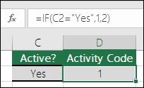Cell D2 contains a formula =IF(C2=

3.1.2. IFS Function

The IFS function has the following syntax:

IFS(logical_test1, value_if_true1, [logical_test2, value_if_true2], ...)

logical_test1: The first condition you want to evaluate.
value_if_true1: The value returned if the first condition is true.
logical_test2, value_if_true2, …: Additional conditions and their corresponding return values.

Example:

=IFS(A1>90, "A", A1>80, "B", A1>70, "C", TRUE, "D")

This formula checks multiple conditions: if A1 is greater than 90, it returns “A”; if A1 is greater than 80, it returns “B”; if A1 is greater than 70, it returns “C”; otherwise, it returns “D”.

3.1.3. Key Differences

Multiple Conditions: IFS can handle multiple conditions in a single function, while IF requires nested statements for multiple conditions.
Readability: IFS is generally more readable and easier to maintain than nested IF statements.
Availability: IFS is only available in Excel 2016 and later versions.

3.1.4. When to Use Each Function

Use IF for simple conditions with one or two outcomes.
Use IFS for multiple conditions where readability and simplicity are important.

3.2. AND vs. OR

The AND and OR functions are used to combine multiple logical conditions. AND returns TRUE if all conditions are true, while OR returns TRUE if at least one condition is true.

3.2.1. AND Function

The AND function has the following syntax:

AND(logical1, [logical2], ...)

logical1, logical2, …: The conditions you want to evaluate.

Example:

=AND(A1>0, B1<100)

This formula checks if A1 is greater than 0 AND B1 is less than 100. It returns TRUE only if both conditions are met.

3.2.2. OR Function

The OR function has the following syntax:

OR(logical1, [logical2], ...)

logical1, logical2, …: The conditions you want to evaluate.

Example:

=OR(A1<0, B1>100)

This formula checks if A1 is less than 0 OR B1 is greater than 100. It returns TRUE if either condition is met.

3.2.3. Key Differences

Condition Requirement: AND requires all conditions to be true, while OR requires at least one condition to be true.
Use Cases: AND is used when you need to ensure all criteria are met, while OR is used when any of the criteria can be met.

3.2.4. When to Use Each Function

Use AND when you need to combine multiple conditions that all must be true.
Use OR when you need to combine multiple conditions where at least one must be true.

3.3. NOT Function

The NOT function is used to reverse the value of a logical expression. If the expression is TRUE, NOT returns FALSE, and vice versa.

3.3.1. NOT Function Syntax

The NOT function has the following syntax:

NOT(logical)

logical: The condition you want to reverse.

Example:

=NOT(A1>50)

This formula checks if A1 is NOT greater than 50. If A1 is less than or equal to 50, it returns TRUE.

3.3.2. Use Cases

Inverting Conditions: NOT is useful for inverting conditions in complex logical expressions.
Simplifying Formulas: It can sometimes simplify formulas by reversing the logic.

3.3.3. When to Use the NOT Function

Use NOT when you need to reverse the outcome of a logical test.

4. Common Mathematical Functions Comparison

Mathematical functions are used to perform calculations on numerical data.

4.1. SUM vs. SUMIF vs. SUMIFS

The SUM function adds up a range of numbers. SUMIF sums values based on a single criterion, while SUMIFS sums values based on multiple criteria.

4.1.1. SUM Function

The SUM function has the following syntax:

SUM(number1, [number2], ...)

number1, number2, …: The numbers you want to add.

Example:

=SUM(A1:A10)

This formula adds up the numbers in cells A1 through A10.

4.1.2. SUMIF Function

The SUMIF function has the following syntax:

SUMIF(range, criteria, [sum_range])

range: The range of cells you want to evaluate.
criteria: The condition that determines which cells to add.
sum_range: The range of cells to sum. If omitted, the range is summed.

Example:

=SUMIF(B1:B10, ">0", A1:A10)

This formula sums the values in A1:A10 where the corresponding value in B1:B10 is greater than 0.

4.1.3. SUMIFS Function

The SUMIFS function has the following syntax:

SUMIFS(sum_range, criteria_range1, criteria1, [criteria_range2, criteria2], ...)

sum_range: The range of cells to sum.
criteria_range1: The first range of cells to evaluate.
criteria1: The first condition that determines which cells to add.
criteria_range2, criteria2, …: Additional ranges and conditions.

Example:

=SUMIFS(A1:A10, B1:B10, ">0", C1:C10, "<100")

This formula sums the values in A1:A10 where the corresponding value in B1:B10 is greater than 0 AND the corresponding value in C1:C10 is less than 100.

4.1.4. Key Differences

Criteria: SUM adds all numbers in a range, SUMIF adds numbers based on one criterion, and SUMIFS adds numbers based on multiple criteria.
Syntax: SUMIF and SUMIFS have different syntax to accommodate their respective criteria.

4.1.5. When to Use Each Function

Use SUM to add up a range of numbers without any conditions.
Use SUMIF to add up numbers based on a single condition.
Use SUMIFS to add up numbers based on multiple conditions.

4.2. AVERAGE vs. AVERAGEIF vs. AVERAGEIFS

The AVERAGE function calculates the average of a range of numbers. AVERAGEIF calculates the average based on a single criterion, while AVERAGEIFS calculates the average based on multiple criteria.

4.2.1. AVERAGE Function

The AVERAGE function has the following syntax:

AVERAGE(number1, [number2], ...)

number1, number2, …: The numbers you want to average.

Example:

=AVERAGE(A1:A10)

This formula calculates the average of the numbers in cells A1 through A10.

4.2.2. AVERAGEIF Function

The AVERAGEIF function has the following syntax:

AVERAGEIF(range, criteria, [average_range])

range: The range of cells you want to evaluate.
criteria: The condition that determines which cells to average.
average_range: The range of cells to average. If omitted, the range is averaged.

Example:

=AVERAGEIF(B1:B10, ">0", A1:A10)

This formula calculates the average of the values in A1:A10 where the corresponding value in B1:B10 is greater than 0.

4.2.3. AVERAGEIFS Function

The AVERAGEIFS function has the following syntax:

AVERAGEIFS(average_range, criteria_range1, criteria1, [criteria_range2, criteria2], ...)

average_range: The range of cells to average.
criteria_range1: The first range of cells to evaluate.
criteria1: The first condition that determines which cells to average.
criteria_range2, criteria2, …: Additional ranges and conditions.

Example:

=AVERAGEIFS(A1:A10, B1:B10, ">0", C1:C10, "<100")

This formula calculates the average of the values in A1:A10 where the corresponding value in B1:B10 is greater than 0 AND the corresponding value in C1:C10 is less than 100.

4.2.4. Key Differences

Criteria: AVERAGE averages all numbers in a range, AVERAGEIF averages numbers based on one criterion, and AVERAGEIFS averages numbers based on multiple criteria.
Syntax: AVERAGEIF and AVERAGEIFS have different syntax to accommodate their respective criteria.

4.2.5. When to Use Each Function

Use AVERAGE to calculate the average of a range of numbers without any conditions.
Use AVERAGEIF to calculate the average of numbers based on a single condition.
Use AVERAGEIFS to calculate the average of numbers based on multiple conditions.

4.3. COUNT vs. COUNTA vs. COUNTIF vs. COUNTIFS

The COUNT function counts the number of cells that contain numbers. COUNTA counts the number of cells that are not empty. COUNTIF counts cells based on a single criterion, while COUNTIFS counts cells based on multiple criteria.

4.3.1. COUNT Function

The COUNT function has the following syntax:

COUNT(value1, [value2], ...)

value1, value2, …: The values or ranges you want to count.

Example:

=COUNT(A1:A10)

This formula counts the number of cells in A1 through A10 that contain numbers.

4.3.2. COUNTA Function

The COUNTA function has the following syntax:

COUNTA(value1, [value2], ...)

value1, value2, …: The values or ranges you want to count.

Example:

=COUNTA(A1:A10)

This formula counts the number of cells in A1 through A10 that are not empty.

4.3.3. COUNTIF Function

The COUNTIF function has the following syntax:

COUNTIF(range, criteria)

range: The range of cells you want to evaluate.
criteria: The condition that determines which cells to count.

Example:

=COUNTIF(B1:B10, ">0")

This formula counts the number of cells in B1 through B10 that are greater than 0.

4.3.4. COUNTIFS Function

The COUNTIFS function has the following syntax:

COUNTIFS(criteria_range1, criteria1, [criteria_range2, criteria2], ...)

criteria_range1: The first range of cells to evaluate.
criteria1: The first condition that determines which cells to count.
criteria_range2, criteria2, …: Additional ranges and conditions.

Example:

=COUNTIFS(B1:B10, ">0", C1:C10, "<100")

This formula counts the number of cells where the corresponding value in B1:B10 is greater than 0 AND the corresponding value in C1:C10 is less than 100.

4.3.5. Key Differences

Content Type: COUNT counts only numbers, COUNTA counts any non-empty cells, and COUNTIF and COUNTIFS count cells based on specified criteria.
Criteria: COUNTIF counts based on one criterion, and COUNTIFS counts based on multiple criteria.

4.3.6. When to Use Each Function

Use COUNT to count the number of cells containing numbers.
Use COUNTA to count the number of non-empty cells.
Use COUNTIF to count cells based on a single condition.
Use COUNTIFS to count cells based on multiple conditions.

5. Text Functions Comparison

Text functions are used to manipulate and analyze text data.

5.1. LEFT vs. RIGHT vs. MID

The LEFT function extracts a specified number of characters from the beginning of a text string. The RIGHT function extracts characters from the end, and the MID function extracts characters from the middle.

5.1.1. LEFT Function

The LEFT function has the following syntax:

LEFT(text, [num_chars])

text: The text string from which you want to extract characters.
num_chars: The number of characters you want to extract from the beginning of the string.

Example:

=LEFT("Hello World", 5)

This formula extracts the first 5 characters from the string “Hello World”, returning “Hello”.

5.1.2. RIGHT Function

The RIGHT function has the following syntax:

RIGHT(text, [num_chars])

text: The text string from which you want to extract characters.
num_chars: The number of characters you want to extract from the end of the string.

Example:

=RIGHT("Hello World", 5)

This formula extracts the last 5 characters from the string “Hello World”, returning “World”.

5.1.3. MID Function

The MID function has the following syntax:

MID(text, start_num, num_chars)

text: The text string from which you want to extract characters.
start_num: The position of the first character you want to extract.
num_chars: The number of characters you want to extract.

Example:

=MID("Hello World", 7, 5)

This formula extracts 5 characters from the string “Hello World”, starting from the 7th character, returning “World”.

5.1.4. Key Differences

Extraction Point: LEFT extracts from the beginning, RIGHT extracts from the end, and MID extracts from a specified position.
Arguments: MID requires a start position, while LEFT and RIGHT do not.

5.1.5. When to Use Each Function

Use LEFT to extract characters from the beginning of a text string.
Use RIGHT to extract characters from the end of a text string.
Use MID to extract characters from a specific position in a text string.

5.2. CONCATENATE vs. TEXTJOIN

The CONCATENATE function joins two or more text strings into one string. TEXTJOIN also joins text strings but allows you to specify a delimiter and ignore empty cells.

5.2.1. CONCATENATE Function

The CONCATENATE function has the following syntax:

CONCATENATE(text1, [text2], ...)

text1, text2, …: The text strings you want to join.

Example:

=CONCATENATE("Hello", " ", "World")

This formula joins the strings “Hello”, ” “, and “World”, returning “Hello World”.

5.2.2. TEXTJOIN Function

The TEXTJOIN function has the following syntax:

TEXTJOIN(delimiter, ignore_empty, text1, [text2], ...)

delimiter: The character(s) you want to insert between the text strings.
ignore_empty: TRUE to ignore empty cells; FALSE to include them.
text1, text2, …: The text strings you want to join.

Example:

=TEXTJOIN(" ", TRUE, "Hello", "", "World")

This formula joins the strings “Hello”, “”, and “World” with a space delimiter, ignoring the empty string, returning “Hello World”.

5.2.3. Key Differences

Delimiter: TEXTJOIN allows you to specify a delimiter, while CONCATENATE does not.
Empty Cells: TEXTJOIN can ignore empty cells, while CONCATENATE includes them.
Availability: TEXTJOIN is available in Excel 2016 and later versions.

5.2.4. When to Use Each Function

Use CONCATENATE to join text strings without a delimiter and when you need to include empty cells.
Use TEXTJOIN to join text strings with a delimiter and when you want to ignore empty cells.

5.3. FIND vs. SEARCH

The FIND function returns the starting position of one text string within another, case-sensitive. The SEARCH function does the same but is not case-sensitive and allows wildcard characters.

5.3.1. FIND Function

The FIND function has the following syntax:

FIND(find_text, within_text, [start_num])

find_text: The text you want to find.
within_text: The text in which you want to search.
start_num: The position at which to start the search (optional).

Example:

=FIND("World", "Hello World")

This formula finds the starting position of “World” within “Hello World”, returning 7.

5.3.2. SEARCH Function

The SEARCH function has the following syntax:

SEARCH(find_text, within_text, [start_num])

find_text: The text you want to find.
within_text: The text in which you want to search.
start_num: The position at which to start the search (optional).

Example:

=SEARCH("world", "Hello World")

This formula finds the starting position of “world” within “Hello World”, returning 7 (case-insensitive).

5.3.3. Key Differences

Case Sensitivity: FIND is case-sensitive, while SEARCH is not.
Wildcards: SEARCH allows wildcard characters (* and ?), while FIND does not.

5.3.4. When to Use Each Function

Use FIND when you need a case-sensitive search and don’t need wildcard characters.
Use SEARCH when you need a case-insensitive search or want to use wildcard characters.

6. Date and Time Functions Comparison

Date and time functions are used to work with date and time values.

6.1. DATE vs. DATEVALUE

The DATE function returns a date given year, month, and day. The DATEVALUE function converts a date in text format to a serial date number.

6.1.1. DATE Function

The DATE function has the following syntax:

DATE(year, month, day)

year: The year.
month: The month.
day: The day.

Example:

=DATE(2024, 1, 1)

This formula returns the date January 1, 2024.

6.1.2. DATEVALUE Function

The DATEVALUE function has the following syntax:

DATEVALUE(date_text)

date_text: The date in text format.

Example:

=DATEVALUE("January 1, 2024")

This formula converts the text “January 1, 2024” to a serial date number.

6.1.3. Key Differences

Input Type: DATE takes numerical inputs for year, month, and day, while DATEVALUE takes a text input representing a date.
Output Type: DATE returns a date, while DATEVALUE returns a serial date number.

6.1.4. When to Use Each Function

Use DATE when you have the year, month, and day as separate numbers.
Use DATEVALUE when you have a date in text format that you need to convert to a serial date number for calculations.

6.2. TODAY vs. NOW

The TODAY function returns the current date. The NOW function returns the current date and time.

6.2.1. TODAY Function

The TODAY function has the following syntax:

TODAY()

Example:

=TODAY()

This formula returns the current date.

6.2.2. NOW Function

The NOW function has the following syntax:

NOW()

Example:

=NOW()

This formula returns the current date and time.

6.2.3. Key Differences

Time Component: TODAY returns only the date, while NOW returns both the date and time.

6.2.4. When to Use Each Function

Use TODAY when you only need the current date.
Use NOW when you need both the current date and time.

6.3. YEAR vs. MONTH vs. DAY

The YEAR function returns the year of a date. The MONTH function returns the month, and the DAY function returns the day.

6.3.1. YEAR Function

The YEAR function has the following syntax:

YEAR(serial_number)

serial_number: The date from which you want to extract the year.

Example:

=YEAR("1/1/2024")

This formula returns the year 2024.

6.3.2. MONTH Function

The MONTH function has the following syntax:

MONTH(serial_number)

serial_number: The date from which you want to extract the month.

Example:

=MONTH("1/1/2024")

This formula returns the month 1 (January).

6.3.3. DAY Function

The DAY function has the following syntax:

DAY(serial_number)

serial_number: The date from which you want to extract the day.

Example:

=DAY("1/1/2024")

This formula returns the day 1.

6.3.4. Key Differences

Extracted Component: Each function extracts a different component of a date (year, month, or day).

6.3.5. When to Use Each Function

Use YEAR to extract the year from a date.
Use MONTH to extract the month from a date.
Use DAY to extract the day from a date.

7. Lookup and Reference Functions Comparison

Lookup and reference functions are used to find values in a table or range.

7.1. VLOOKUP vs. HLOOKUP

The VLOOKUP function looks for a value in the first column of a table and returns a value from the same row in a specified column. The HLOOKUP function does the same but looks in the first row of a table and returns a value from the same column in a specified row.

7.1.1. VLOOKUP Function

The VLOOKUP function has the following syntax:

VLOOKUP(lookup_value, table_array, col_index_num, [range_lookup])

lookup_value: The value you want to look for.
table_array: The table in which you want to look.
col_index_num: The column number from which to return a value.
range_lookup: TRUE for an approximate match (default), FALSE for an exact match.

Example:

=VLOOKUP("Apple", A1:C10, 2, FALSE)

This formula looks for “Apple” in the first column of the table A1:C10 and returns the value from the second column in the same row, requiring an exact match.

7.1.2. HLOOKUP Function

The HLOOKUP function has the following syntax:

HLOOKUP(lookup_value, table_array, row_index_num, [range_lookup])

lookup_value: The value you want to look for.
table_array: The table in which you want to look.
row_index_num: The row number from which to return a value.
range_lookup: TRUE for an approximate match (default), FALSE for an exact match.

Example:

=HLOOKUP("Apple", A1:C10, 2, FALSE)

This formula looks for “Apple” in the first row of the table A1:C10 and returns the value from the second row in the same column, requiring an exact match.

7.1.3. Key Differences

Orientation: VLOOKUP looks vertically (in columns), while HLOOKUP looks horizontally (in rows).
Row vs. Column: VLOOKUP returns a value from a specified column, while HLOOKUP returns a value from a specified row.

7.1.4. When to Use Each Function

Use VLOOKUP when your lookup table is arranged vertically.
Use HLOOKUP when your lookup table is arranged horizontally.

7.2. INDEX vs. MATCH

The INDEX function returns a value from a table based on row and column numbers. The MATCH function returns the position of a value in a range.

7.2.1. INDEX Function

The INDEX function has the following syntax:

INDEX(array, row_num, [column_num])

array: The range of cells from which you want to return a value.
row_num: The row number from which to return a value.
column_num: The column number from which to return a value (optional).

Example:

=INDEX(A1:C10, 5, 2)

This formula returns the value from the 5th row and 2nd column of the range A1:C10.

7.2.2. MATCH Function

The MATCH function has the following syntax:

MATCH(lookup_value, lookup_array, [match_type])

lookup_value: The value you want to find.
lookup_array: The range of cells you want to search.
match_type: 1 for less than, 0 for exact match, -1 for greater than (optional).

Example:

=MATCH("Apple", A1:A10, 0)

This formula finds the position of “Apple” in the range A1:A10, requiring an exact match.

7.2.3. Key Differences

Purpose: INDEX returns a value from a specified location, while MATCH returns the position of a value.
Arguments: INDEX requires row and column numbers, while MATCH requires a lookup value and array.

7.2.4. When to Use Each Function

Use INDEX when you know the row and column numbers of the value you want to retrieve.
Use MATCH when you need to find the position of a value in a range.

7.3. CHOOSE Function

The CHOOSE function returns a value from a list of values based on an index number.

7.3.1. CHOOSE Function Syntax

The CHOOSE function has the following syntax:

CHOOSE(index_num, value1, [value2], ...)

index_num: The index number (1, 2, 3, …) that specifies which value to return.
value1, value2, …: The list of values from which to choose.

Example:

=CHOOSE(2, "Apple", "Banana", "Cherry")

This formula returns the second value in the list, which is “Banana”.

7.3.2. Use Cases

Selecting from a List: CHOOSE is useful for selecting one value from a predefined list based on an index number.
Dynamic Formulas: It can be used to create dynamic formulas that change based on the index number.

7.3.3. When to Use the CHOOSE Function

Use CHOOSE when you need to select one value from a list based on an index number.

8. Statistical Functions Comparison

Statistical functions are used to perform statistical analysis on data.

8.1. STDEV.S vs. STDEV.P

The STDEV.S function calculates the sample standard deviation. The STDEV.P function calculates the population standard deviation.

8.1.1. STDEV.S Function

The STDEV.S function has the following syntax:

STDEV.S(number1, [number2], ...)

number1, number2, …: The numbers representing a sample of a population.

Example:

=STDEV.S(A1:A10)

This formula calculates the sample standard deviation of the numbers in A1:A10.

8.1.2. STDEV.P Function

The STDEV.P function has the following syntax:

STDEV.P(number1, [number2], ...)

number1, number2, …: The numbers representing the entire population.

Example:

=STDEV.P(A1:A10)

This formula calculates the population standard deviation of the numbers in A1:A10.

8.1.3. Key Differences

Data Representation: STDEV.S is used when the data represents a sample of a population, while STDEV.P is used when the data represents the entire population.
Calculation: The formulas differ slightly in their calculations to account for whether the data is a sample or the entire population.

8.1.4. When to Use Each Function

Use STDEV.S when you are working with a sample of a population.
Use STDEV.P when you are working with the entire population.

8.2. VAR.S vs. VAR.P

The VAR.S function calculates the sample variance. The VAR.P function calculates the population variance.

8.2.1. VAR.S Function

The