How To Compare The Columns In Excel: A Comprehensive Guide

Comparing columns in Excel can be a game-changer for data analysis, and COMPARE.EDU.VN offers a comprehensive guide to help you master this skill. Learn how to identify matching or differing data efficiently using various methods, from simple formulas to advanced conditional formatting. Master the art of data comparison with these effective Excel techniques, including identifying data discrepancies and utilizing lookup functions.

1. Why Comparing Columns In Excel Is Essential?

Excel is more than just a spreadsheet; it’s a powerful tool for data storage, analysis, and informed decision-making. A key feature that empowers data analysts is the ability to compare two columns. This allows for the identification of similarities and differences across the same or different spreadsheets. Manually comparing columns, especially in large datasets, is a time-consuming and error-prone task. Comparing columns in Excel is crucial for determining the presence or absence of specific data, flagging discrepancies, and ensuring data integrity.

2. What Are The Common Methods To Compare Columns In Excel?

Comparing columns in Excel unlocks valuable insights from your data, revealing matches, discrepancies, and unique entries across different datasets. Several methods can be used to compare data in Excel columns, each serving a specific purpose:

Highlighting Unique or Duplicate Values: Identify distinct entries or common data points across columns.
Conditional Formatting: Visually flag matching or mismatching cells based on predefined criteria.
Row-by-Row Comparison: Compare corresponding cells in each row to identify differences.
Lookup Formulas: Search for specific values in one column and retrieve related information from another.

3. How To Compare Two Columns In Excel Using The Equals Operator?

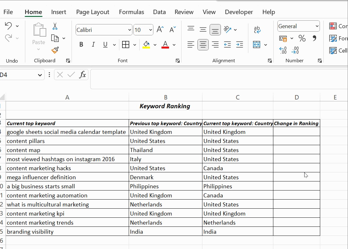
The equals operator (=) provides a straightforward method for performing a row-by-row comparison of two columns, highlighting matching data with a “True” result and differences with a “False” result. You can compare two columns on a row-by-row basis, displaying either “Match” or “Not Match” based on whether the data is the same. Excel defaults to displaying “True” if there is a match and “False” otherwise.

In cell D4, input the formula =B4=C4 and then press Enter.
Pull it downwards towards the bottom of the table.
If the compared columns have the same values, the formula will return TRUE; if the values are different, it will return FALSE.

4. How To Compare Two Columns In Excel Using The IF Condition?

The IF condition introduces flexibility by allowing you to define custom results for matches and mismatches. With the IF condition in Excel, you can compare two columns and receive a “Yes” or other customized response for matching values.

The formula to compare two columns is =IF(B4=C4,”Yes”,” ”). This returns “Yes” for rows with matching values and leaves the remaining rows empty.

To identify and return mismatching values, include an additional argument, “No,” when the IF condition proves false. The formula becomes =IF(B4=C4,”Yes”,”No”).

To compare two columns for differences, replace the equals sign with the non-equality sign (<>). The formula is =IF(A2<>B2,”Match”,”Not a Match ”).

5. How To Compare Two Columns In Excel Using The EXACT() Function?

The EXACT() function refines the comparison by ensuring that both the values and the capitalization match, offering a case-sensitive comparison. When comparing two Excel columns and IF(), use EXACT() to ensure that the capitalizations are identical.

The EXACT() function compares two text strings and returns Yes only if they have the same capitalization. EXACT is case-sensitive but ignores formatting differences. The syntax is =EXACT(text1,text2). It takes two arguments, text1 and text2; both are required when using this function.

Use the formula =IF(EXACT(B4,C4), “Match”, “Mismatched”) for the IF condition to be case-sensitive.

It returns a result of “Mismatched” for columns with matching results yet mismatched capitalizations.

6. How Does The EXACT() Function Work?

The EXACT() function works by comparing two text strings character by character, returning TRUE only if they are identical, including case. The first thing that happens when the formula is run is that the inner function runs and returns the result. EXACT() function returns a false value to the outer function IF.

The general working of the IF condition is that if it returns true, the first argument in the function is returned. Or the second argument is returned as false.

7. How To Compare Two Columns In Excel Using Conditional Formatting?

Conditional formatting visually highlights matching or differing data, making it easy to identify patterns and anomalies. Conditional formatting helps find and highlight data present in both columns. Select the columns to compare before using conditional formatting.

Click Home, then on Styles.

Then, follow these steps Conditional Formatting → Highlight Cell Rules → Duplicate Values.

You get a dialogue box, as shown below. From there, you must choose the values from the drop-down menu.

Apply the formatting condition on the cells. You can choose any conditions; Duplicate or Unique.

Format cells that contain: (options) values with (options).

Choose Duplicate if you wish to find the names in both columns. To highlight it, choose any options: filling with color, changing the text color, or changing the cell border.

The last option is a Custom Format. Choose this option if you wish to highlight the cell with a color of your choice other than the ones specified in the drop-down menu.

Another option that you can use is “Unique.” Use this option if you are interested in highlighting the cells that contain data that is not repeated. That is, you wish to highlight the unique cells.

Instead of selecting Duplicate, choose Unique from the drop-down list, and apply any options, such as filling with color, changing the text color, or changing the cell border.

Tip: If you wish to clear the formatting you performed on the cells, click Conditional Formatting → Clear Rules → Clear Rules from Selected Cells.

When you don’t want a third column showing the results comparing the two columns, you can use conditional formatting. Highlighting duplicate (matching) and unique (different) data shows which rows have the same data.

Additionally, you can use an extra column to explicitly display values indicating whether the data matches, which works for smaller tables. Alternatively, you may need to use more complex methods for large spreadsheets.

8. How To Use The Lookup Function To Compare Two Columns?

Lookup functions enable you to search for specific values in one column and retrieve corresponding values from another, facilitating comparisons and data retrieval. The LOOKUP function searches for a particular value in a row or column and returns the corresponding value from another row or column. There are various lookup functions, viz, HLOOKUP, VLOOKUP, and XLOOKUP, where H and V stand for horizontal and vertical, and the XLOOKUP function is a combination of both LOOKUP and VLOOKUP.

The example below is to compare two columns in Excel for differences using VLOOKUP().

Column A contains a list of top keywords in a blog, and column B is the parent keyword. The resulting comparison must return all the ranking keywords in the blog.

The VLOOKUP() is applied in cell C4 as =VLOOKUP(A4, £B£4:£B£15,1,0).

Drag the cell to apply the formula in all the cells below C4. You will find the result in column C with the current and the matching parent keywords. The formula in Excel to compare two columns using VLOOKUP is as follows.

VLOOKUP(A4,..,..,..) – This takes the value in cell A4.

VLOOKUP(A4, £B£4:£B£15,..,..) – This compares all the values in cells from B4 to B15. That’s why the cells in range B4:B15 are locked using absolute reference. The £ symbol before the cell reference is called an absolute reference.

VLOOKUP(A4, £B£4:£B£15,1,..) – The third argument is the col_index_num, which mentions the position of the column to compare from the lookup value A4.

In the above example, the current top keyword is in column A, and the column with which it has to be compared is 1 column away. Hence, the value 1.

VLOOKUP(A4, £B£4:£B£15,1,0) – The last argument takes a logical value, either 0 or 1.

If you wish to find the exact match, mention 0(zero). If you want VLOOKUP() to return a closet match sorted in ascending order, mention 1 in this argument.

9. How To Compare Data With VLOOKUP()?

VLOOKUP() compares the value in a specified cell to a range of cells, returning a corresponding value from the same row in another column. VLOOKUP(A4,..,..,..) – This takes the value in cell A4.

VLOOKUP(A4, £B£4:£B£15,1,..) – The third argument is the col_index_num, which mentions the position of the column to compare from the lookup value A4.

VLOOKUP(A4, £B£4:£B£15,1,0) – The last argument takes a logical value, either 0 or 1.

10. What Are Absolute References?

Absolute references, denoted by the £ symbol, lock a cell reference, preventing it from changing when the formula is copied to other cells. The £ symbol before the cell reference is called an absolute reference.

11. What Is The Difference Between HLOOKUP And VLOOKUP?

HLOOKUP searches horizontally across the top row of a table and retrieves a value from a specified row, while VLOOKUP searches vertically down the first column of a table and retrieves a value from a specified column. H and V stand for horizontal and vertical, and the XLOOKUP function is a combination of both LOOKUP and VLOOKUP.

12. What Is The XLOOKUP Function?

XLOOKUP is a modern lookup function that combines the capabilities of both HLOOKUP and VLOOKUP, offering greater flexibility and ease of use. The XLOOKUP function is a combination of both LOOKUP and VLOOKUP.

13. How To Compare Three Or More Columns In Excel?

For comparing three or more columns, Excel provides formulas that can identify matches across all or any of the specified columns. When the table has three or more columns, use an IF() with AND statement to find matches in all cells. The formula is =IF(AND(A2=B2, A2=C2), “Full match”, “”).

The formula to find matches in any two cells in the same row is =IF(OR(A2=B2, B2=C2, A2=C2), “Match”, “”).

14. How To Find Row Differences In Excel?

To find row differences, select both columns of data, then navigate to Home → Find & Select → Go To Special → Row Differences, and click OK. Unmatched cells appear in gray, while matching data cells are white.

15. Can The Methods Described Be Used With Different Versions Of Excel?

Yes, the methods described are generally applicable across different versions of Excel, although minor interface differences may exist.

16. Can I Compare Columns With Different Data Types (E.G., Text And Numbers)?

Yes, Excel allows you to compare columns with different data types, but be mindful of potential conversion issues and ensure appropriate formatting.

17. How Do I Handle Errors When Comparing Columns In Excel?

When comparing columns in Excel, handling errors gracefully is crucial for maintaining data integrity and ensuring accurate analysis. Excel provides built-in functions and techniques to manage errors that may arise during the comparison process. Here’s a guide on how to handle errors effectively:

Understanding Common Error Types:
- #N/A Error: This error typically occurs when using lookup functions like VLOOKUP or HLOOKUP, indicating that a value was not found in the specified range.
- #VALUE! Error: This error arises when a formula contains an argument of the wrong type, such as attempting to perform arithmetic operations on text values.
- #DIV/0! Error: This error occurs when a formula attempts to divide a number by zero or an empty cell.
- #REF! Error: This error indicates that a cell reference in a formula is no longer valid, often due to deleting or moving referenced cells.
Using the IFERROR Function:

The IFERROR function is a versatile tool for handling errors in Excel. It allows you to specify an alternative value to return if a formula results in an error. The syntax for IFERROR is as follows:
```
=IFERROR(value, value_if_error)
```
- value: The formula or expression to evaluate.
- value_if_error: The value to return if the formula results in an error.
- For example, if you’re using VLOOKUP to compare columns and want to return “Not Found” instead of #N/A when a value is not found, you can use the following formula:
```
=IFERROR(VLOOKUP(A1,B:C,2,FALSE), "Not Found")
```
Using Conditional Formatting with Error Handling:

You can combine conditional formatting with error handling to visually highlight cells that contain errors. This allows you to quickly identify and address errors in your data.
- Select the range of cells you want to format.
- Go to Home > Conditional Formatting > New Rule.
- Choose “Use a formula to determine which cells to format.”
- Enter a formula that checks for errors using functions like ISERROR, ISNA, or ISBLANK.
- For example, to highlight cells containing any type of error, use the following formula:
```
=ISERROR(A1)
```
Using the ISERROR, ISNA, and ISBLANK Functions:

Excel provides functions to specifically check for different types of errors:
- ISERROR(value): Returns TRUE if value is any type of error (#N/A, #VALUE!, #DIV/0!, #REF!, etc.).
- ISNA(value): Returns TRUE if value is the #N/A error.
- ISBLANK(value): Returns TRUE if value is an empty cell.
Combining Error Handling with Formula Logic:

You can incorporate error handling directly into your formulas to handle specific error conditions. For example, if you’re dividing two columns and want to avoid the #DIV/0! error, you can use the following formula:
```
=IF(B1=0, "Undefined", A1/B1)
```
Data Validation:

You can use data validation to prevent errors from occurring in the first place. Data validation allows you to define rules for what type of data can be entered into a cell, reducing the likelihood of errors.
- Select the range of cells you want to validate.
- Go to Data > Data Validation.
- Set criteria for allowed values, such as data type, range, or list.
- Customize error messages to provide helpful feedback to users when they enter invalid data.
Testing and Debugging:

Before deploying your formulas, it’s essential to test them thoroughly with different scenarios and edge cases. Use sample data to identify potential errors and refine your error-handling techniques.

By implementing these error-handling techniques, you can ensure that your Excel comparisons are robust, accurate, and reliable, even when encountering errors in your data.

18. Can I Automate The Comparison Process With Macros Or VBA?

Yes, you can automate the comparison process using macros or VBA (Visual Basic for Applications) to handle large datasets or repetitive tasks efficiently.

19. How To Ensure Data Integrity During The Comparison Process?

To ensure data integrity during the comparison process, verify data accuracy, standardize formats, and implement data validation rules.

20. What Are Some Advanced Techniques For Comparing Columns In Excel?

Some advanced techniques for comparing columns in Excel include using array formulas, regular expressions, and specialized add-ins.

FAQ: Frequently Asked Questions

1. How do you compare two columns in Excel?

One way to compare two columns in Excel is to select both data columns, select Home → Find & Select → Go To Special → Row Differences, and click OK. The matching data cells across the columns’ rows are white, and unmatched cells appear in gray.

2. How to compare three or more columns in Excel?

To find matches in all cells when the table has three or more columns, use an IF() with AND statement. The formula is =IF(AND(A2=B2, A2=C2), “Full match”, “”).

The formula to find matches in any two cells in the same row is =IF(OR(A2=B2, B2=C2, A2=C2), “Match”, “”).

3. Is the EXACT function case-sensitive?

Yes, the EXACT function is case-sensitive. It will only return “TRUE” if the text in both cells is exactly the same, including capitalization.

4. Can conditional formatting highlight multiple differences between columns?

Yes, conditional formatting can be used to highlight multiple differences between columns by creating multiple rules based on different criteria.

5. What is the purpose of the VLOOKUP function?

The VLOOKUP function is used to search for a value in the first column of a range and then return a value from a specified column in the same row.

6. Can I use wildcards with the VLOOKUP function?

Yes, you can use wildcards with the VLOOKUP function to perform partial matches. For example, you can use the asterisk (*) to match any sequence of characters.

7. What is the difference between relative and absolute cell references?

Relative cell references change when a formula is copied to another cell, while absolute cell references remain constant regardless of where the formula is copied.

8. How can I prevent errors when comparing columns in Excel?

You can prevent errors by ensuring that your data is clean and consistent, using appropriate formulas, and testing your formulas thoroughly.

9. Can I compare columns from different Excel files?

Yes, you can compare columns from different Excel files by referencing the other file in your formulas.

10. How do I clear conditional formatting rules?

To clear conditional formatting rules, select the cells with the formatting, then go to Conditional Formatting → Clear Rules → Clear Rules from Selected Cells.

Conclusion

Comparing columns in Excel is a fundamental skill for data analysis. Excel offers various methods to compare and match data in a single column, multiple columns, and multiple spreadsheets. From simple formulas to advanced techniques, Excel provides the tools necessary to effectively compare data and gain valuable insights. At COMPARE.EDU.VN, we understand the importance of efficient data comparison.

Want to simplify your data analysis and make informed decisions faster? Visit COMPARE.EDU.VN today! Our comprehensive guides and resources will equip you with the Excel skills you need to excel.

Need help with your data comparison tasks? Contact us at:

Address: 333 Comparison Plaza, Choice City, CA 90210, United States.
Whatsapp: +1 (626) 555-9090
Website: compare.edu.vn