Comparing data between two sheets in Excel can be straightforward. compare.edu.vn simplifies this process, offering several effective methods to identify similarities and differences, ensuring data integrity and accuracy. This article explores different Excel features, conditional formatting, and formulas to streamline data analysis. Learn about the benefits of using Spreadsheet Compare and the Inquire add-in for advanced comparisons.
1. What Are The Key Methods To Compare Data Between Two Sheets In Excel?
Excel provides several methods to compare data between two sheets, each with its strengths. These include using conditional formatting, formulas, and the “View Side by Side” feature. Each method is suited to different scenarios based on the amount and type of data you are comparing.
1.1. Using Conditional Formatting
Conditional formatting is a simple way to highlight differences between two sheets. Select the data range in one sheet, create a new rule using a formula, and compare it against the corresponding range in the second sheet.
1.1.1. Steps to Apply Conditional Formatting
- Select the data range in the first sheet.
- Go to Home > Conditional Formatting > New Rule.
- Choose “Use a formula to determine which cells to format.”
- Enter a formula like
=A1<>Sheet2!A1(adjust cell references accordingly). - Click Format to choose a highlight color.
- Click OK to apply the rule.
1.1.2. Advantages of Conditional Formatting
- Visual Highlighting: Quickly identifies differences with color-coding.
- Easy Setup: Simple steps for basic comparisons.
- Dynamic Updates: Automatically updates when data changes.
1.1.3. Limitations of Conditional Formatting
- Manual Setup: Requires manual setup for each comparison.
- Limited Complexity: Best for simple comparisons; struggles with complex criteria.
- Sheet Dependency: Works best when sheets have similar layouts.
1.2. Using Formulas for Comparison
Excel formulas can perform more complex comparisons. Formulas like IF, EXACT, and VLOOKUP can check for matches, differences, and specific data criteria.
1.2.1. Common Formulas for Data Comparison
=IF(A1=Sheet2!A1, "Match", "Mismatch"): Checks if cell A1 in both sheets is identical.=EXACT(A1, Sheet2!A1): Case-sensitive comparison of cell A1 in both sheets.=VLOOKUP(A1, Sheet2!A:B, 2, FALSE): Searches for A1 in Sheet2 and returns a corresponding value.
1.2.2. How to Implement Formulas
- In a new column, enter the comparison formula.
- Drag the formula down to apply it to all rows.
- Review the results (“Match”, “Mismatch”, or values returned by
VLOOKUP).
1.2.3. Advantages of Using Formulas
- Detailed Results: Provides specific match/mismatch results.
- Complex Criteria: Can handle more intricate comparison rules.
- Customizable: Adaptable to different data layouts and requirements.
1.2.4. Limitations of Using Formulas
- Formula Errors: Incorrect formulas can lead to inaccurate results.
- Manual Input: Requires manual formula creation and adjustment.
- Overwhelming Details: Can produce a large amount of data, making it hard to interpret.
1.3. Using “View Side by Side”
Excel’s “View Side by Side” feature is a simple method to visually compare two sheets. This feature allows you to scroll through both sheets simultaneously, making it easier to spot differences.
1.3.1. Steps to Use “View Side by Side”
- Open both Excel sheets you want to compare.
- Go to the View tab.
- Click View Side by Side.
- Enable Synchronous Scrolling to scroll both sheets together.
1.3.2. Benefits of “View Side by Side”
- Visual Inspection: Easy to spot differences visually.
- Simultaneous Scrolling: Synchronized scrolling makes it easier to compare.
- Simple Setup: Quick and straightforward to set up.
1.3.3. Drawbacks of “View Side by Side”
- Manual Review: Requires manual identification of differences.
- Limited Data: Best suited for small datasets.
- No Highlighting: Doesn’t automatically highlight differences.
1.4. Using Power Query for Advanced Comparison
Power Query, also known as Get & Transform Data, allows you to import data from multiple sources, transform it, and load it into Excel. It’s particularly useful for comparing data from different sheets, workbooks, or even external databases.
1.4.1. Steps to Use Power Query
- Go to Data > Get & Transform Data > From Table/Range to import data from each sheet.
- In the Power Query Editor, append the queries to combine the data.
- Add a custom column to compare the values from the original sheets.
- Load the transformed data back into Excel.
1.4.2. Benefits of Power Query
- Data Transformation: Cleans and transforms data during import.
- Multiple Sources: Imports data from various sources.
- Automated Process: Automates the comparison process.
1.4.3. Drawbacks of Power Query
- Complexity: Requires knowledge of Power Query.
- Setup Time: Initial setup can be time-consuming.
- Resource Intensive: May slow down Excel with large datasets.
1.5. Using the “Spreadsheet Compare” Tool
Microsoft’s Spreadsheet Compare tool, part of Office Professional Plus, generates a detailed report of differences between two Excel files. It identifies changes in formulas, cell formats, and more.
1.5.1. How to Access Spreadsheet Compare
- Open the Start menu.
- Type Spreadsheet Compare and select the application.
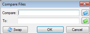
1.5.2. Steps to Compare Files
- Click Compare Files.
- Select the two Excel files to compare.
- Review the detailed comparison report.
1.5.3. Benefits of Using Spreadsheet Compare
- Comprehensive Analysis: Provides a detailed report of all changes.
- Formula Auditing: Identifies differences in formulas.
- Format Comparison: Highlights changes in cell formatting.
1.5.4. Drawbacks of Using Spreadsheet Compare
- Availability: Only available with specific Office versions.
- Complexity: Can be overwhelming for simple comparisons.
- Cost: Requires a specific Office Professional Plus edition.
 Compare Files command
1.6. Utilizing the Inquire Add-In
The Inquire add-in in Excel allows you to analyze workbooks, explore relationships between cells, and identify potential issues. It’s a powerful tool for auditing and ensuring data accuracy.
1.6.1. Enabling the Inquire Add-In
- Go to File > Options > Add-ins.
- In the “Manage” dropdown, select “COM Add-ins” and click Go.
- Check the box next to “Inquire” and click OK.
1.6.2. Key Features of the Inquire Add-In
- Workbook Analysis: Provides an overview of the workbook’s structure.
- Cell Relationships: Shows dependencies between cells.
- Error Checking: Identifies potential errors and inconsistencies.
1.6.3. Benefits of Using the Inquire Add-In
- Comprehensive Analysis: Provides a detailed overview of workbook structure.
- Error Detection: Helps identify potential errors and inconsistencies.
- Enhanced Auditing: Improves the auditing process for Excel files.
1.6.4. Limitations of Using the Inquire Add-In
- Excel Version: Requires a compatible version of Excel.
- Learning Curve: May take time to learn all the features.
- Complexity: Can be overwhelming for simple tasks.
2. How Do I Compare Two Columns In Excel And Highlight The Differences?
To compare two columns in Excel and highlight the differences, you can use conditional formatting with a formula. This method quickly identifies and visually marks the cells that do not match between the two columns.
2.1. Steps to Compare Two Columns
- Select the first column you want to compare.
- Go to Home > Conditional Formatting > New Rule.
- Choose “Use a formula to determine which cells to format.”
- Enter a formula like
=A1<>B1(where A1 is the first cell in the selected column and B1 is the corresponding cell in the second column). - Click Format to choose a highlight color.
- Click OK to apply the rule.
- Repeat for the second column, adjusting the formula as needed (e.g.,
=B1<>A1).
2.2. Example Scenario
Suppose you have two columns, A and B, with customer names. You want to highlight any names that are different in the two columns.
- Select the range
A1:A10. - Go to Conditional Formatting > New Rule.
- Use the formula
=A1<>B1. - Choose a highlight color (e.g., yellow).
- Click OK.
- Select the range
B1:B10. - Go to Conditional Formatting > New Rule.
- Use the formula
=B1<>A1. - Choose a highlight color (e.g., yellow).
- Click OK.
2.3. Advantages of This Method
- Quick Identification: Easily spot differences between columns.
- Visual Cues: Highlighted cells provide immediate visual cues.
- Dynamic Updates: Automatically updates when data changes.
2.4. Limitations
- Manual Setup: Requires manual setup for each comparison.
- Simple Comparisons: Best for basic comparisons; struggles with complex criteria.
- Potential Overlap: If both cells are different, both will be highlighted.
3. Can I Use Excel To Compare Two Lists And Find The Differences?
Yes, Excel can be used to compare two lists and find the differences. Several methods can be used, including conditional formatting, formulas like VLOOKUP and MATCH, and advanced tools like Power Query.
3.1. Using VLOOKUP
The VLOOKUP function can find items in one list that are not in another. It searches for a value in the first column of a range and returns a value in the same row from another column.
3.1.1. Steps to Use VLOOKUP
- Assuming your lists are in columns A and B, in column C, enter the formula
=IF(ISNA(VLOOKUP(A1,B:B,1,FALSE)),"Not Found",""). - Drag the formula down to apply it to all rows in list A.
- Any item in list A that is not found in list B will be marked as “Not Found.”
3.1.2. Advantages of VLOOKUP
- Identifies Missing Items: Quickly finds items in one list that are not in another.
- Easy to Implement: Simple formula for basic comparisons.
- Clear Results: Clearly marks items that are not found.
3.1.3. Limitations of VLOOKUP
- Directional: Only works for finding items in the first column of the lookup range.
- Exact Match: Requires an exact match for accurate results.
- Performance: Can be slow with large datasets.
3.2. Using MATCH
The MATCH function returns the position of a value in a range. It can be used in conjunction with ISNA to find items in one list that are not in another.
3.2.1. Steps to Use MATCH
- Assuming your lists are in columns A and B, in column C, enter the formula
=IF(ISNA(MATCH(A1,B:B,0)),"Not Found",""). - Drag the formula down to apply it to all rows in list A.
- Any item in list A that is not found in list B will be marked as “Not Found.”
3.2.2. Advantages of MATCH
- Precise Matching: Finds exact matches in the specified range.
- Flexible: Can be used with different data types.
- Simple Syntax: Easy to understand and implement.
3.2.3. Limitations of MATCH
- Exact Match Required: Requires an exact match for accurate results.
- Single Column: Only works for single-column ranges.
- Error Handling: Requires error handling (e.g.,
ISNA) to manage non-matches.
3.3. Using Conditional Formatting
Conditional formatting can highlight items in one list that are not in another. This method provides a visual way to identify differences.
3.3.1. Steps to Use Conditional Formatting
- Select the first list (e.g., column A).
- Go to Home > Conditional Formatting > New Rule.
- Choose “Use a formula to determine which cells to format.”
- Enter the formula
=ISNA(MATCH(A1,B:B,0))(where A1 is the first cell in list A and B:B is list B). - Click Format to choose a highlight color.
- Click OK to apply the rule.
3.3.2. Advantages of Conditional Formatting
- Visual Highlighting: Easily identifies differences with color-coding.
- Easy Setup: Simple steps for basic comparisons.
- Dynamic Updates: Automatically updates when data changes.
3.3.3. Limitations of Conditional Formatting
- Manual Setup: Requires manual setup for each comparison.
- Limited Complexity: Best for simple comparisons; struggles with complex criteria.
- Sheet Dependency: Works best when sheets have similar layouts.
3.4. Using Power Query
Power Query can merge and compare lists from different sources. This method is more advanced but very powerful for complex comparisons.
3.4.1. Steps to Use Power Query
- Import both lists into Power Query using Data > From Table/Range.
- Merge the queries using a left anti-join (rows only in the first list).
- Load the resulting data back into Excel.
3.4.2. Advantages of Power Query
- Data Transformation: Cleans and transforms data during import.
- Multiple Sources: Imports data from various sources.
- Automated Process: Automates the comparison process.
3.4.3. Limitations of Power Query
- Complexity: Requires knowledge of Power Query.
- Setup Time: Initial setup can be time-consuming.
- Resource Intensive: May slow down Excel with large datasets.
4. What Is The Best Way To Compare Two Excel Files For Differences?
The best way to compare two Excel files for differences depends on the complexity and scope of the comparison you need. For basic comparisons, conditional formatting or simple formulas might suffice. However, for comprehensive and detailed comparisons, Microsoft’s Spreadsheet Compare tool is generally the most effective method.
4.1. Spreadsheet Compare Tool
The Spreadsheet Compare tool, part of Office Professional Plus, generates a detailed report of differences between two Excel files. It identifies changes in formulas, cell formats, and more.
4.1.1. How to Access Spreadsheet Compare
- Open the Start menu.
- Type Spreadsheet Compare and select the application.
4.1.2. Steps to Compare Files
- Click Compare Files.
- Select the two Excel files to compare.
- Review the detailed comparison report.
4.1.3. Benefits of Using Spreadsheet Compare
- Comprehensive Analysis: Provides a detailed report of all changes.
- Formula Auditing: Identifies differences in formulas.
- Format Comparison: Highlights changes in cell formatting.
4.1.4. Drawbacks of Using Spreadsheet Compare
- Availability: Only available with specific Office versions.
- Complexity: Can be overwhelming for simple comparisons.
- Cost: Requires a specific Office Professional Plus edition.
4.2. Excel’s Inquire Add-In
The Inquire add-in in Excel allows you to analyze workbooks, explore relationships between cells, and identify potential issues. It’s a powerful tool for auditing and ensuring data accuracy.
4.2.1. Enabling the Inquire Add-In
- Go to File > Options > Add-ins.
- In the “Manage” dropdown, select “COM Add-ins” and click Go.
- Check the box next to “Inquire” and click OK.
4.2.2. Key Features of the Inquire Add-In
- Workbook Analysis: Provides an overview of the workbook’s structure.
- Cell Relationships: Shows dependencies between cells.
- Error Checking: Identifies potential errors and inconsistencies.
4.2.3. Benefits of Using the Inquire Add-In
- Comprehensive Analysis: Provides a detailed overview of workbook structure.
- Error Detection: Helps identify potential errors and inconsistencies.
- Enhanced Auditing: Improves the auditing process for Excel files.
4.2.4. Limitations of Using the Inquire Add-In
- Excel Version: Requires a compatible version of Excel.
- Learning Curve: May take time to learn all the features.
- Complexity: Can be overwhelming for simple tasks.
4.3. Power Query for Data Comparison
Power Query, also known as Get & Transform Data, allows you to import data from multiple sources, transform it, and load it into Excel. It’s particularly useful for comparing data from different sheets, workbooks, or even external databases.
4.3.1. Steps to Use Power Query
- Go to Data > Get & Transform Data > From Table/Range to import data from each sheet.
- In the Power Query Editor, append the queries to combine the data.
- Add a custom column to compare the values from the original sheets.
- Load the transformed data back into Excel.
4.3.2. Benefits of Power Query
- Data Transformation: Cleans and transforms data during import.
- Multiple Sources: Imports data from various sources.
- Automated Process: Automates the comparison process.
4.3.3. Drawbacks of Power Query
- Complexity: Requires knowledge of Power Query.
- Setup Time: Initial setup can be time-consuming.
- Resource Intensive: May slow down Excel with large datasets.
4.4. Formulas and Conditional Formatting
For smaller datasets or specific comparisons, formulas and conditional formatting can be effective.
4.4.1. Formulas for Comparison
Use formulas like IF, EXACT, and VLOOKUP to check for matches, differences, and specific data criteria.
4.4.2. Conditional Formatting for Visual Highlighting
Use conditional formatting to highlight differences between two ranges.
5. How Can I Compare Data In Excel And Identify Duplicate Entries?
Identifying duplicate entries in Excel is a common task that can be accomplished using conditional formatting, the COUNTIF function, or the “Remove Duplicates” feature. Each method offers a different approach to finding and managing duplicates.
5.1. Using Conditional Formatting
Conditional formatting can highlight duplicate entries in a range. This method is useful for visually identifying duplicates.
5.1.1. Steps to Use Conditional Formatting
- Select the range of cells you want to check for duplicates.
- Go to Home > Conditional Formatting > Highlight Cells Rules > Duplicate Values.
- Choose the formatting style (e.g., light red fill) and click OK.
5.1.2. Advantages of Conditional Formatting
- Visual Identification: Easily spot duplicates with color-coding.
- Simple Setup: Quick and straightforward to set up.
- Dynamic Updates: Automatically updates when data changes.
5.1.3. Limitations of Conditional Formatting
- Doesn’t Remove Duplicates: Only highlights them.
- Limited Customization: Formatting options are limited.
- Manual Action: Requires manual action to remove or manage duplicates.
5.2. Using the COUNTIF Function
The COUNTIF function counts the number of cells within a range that meet a given criterion. It can be used to identify duplicate entries by counting how many times each entry appears in the range.
5.2.1. Steps to Use COUNTIF
- In a new column, enter the formula
=COUNTIF(A:A, A1)(where A:A is the range of cells and A1 is the first cell in the range). - Drag the formula down to apply it to all rows.
- Any cell with a count greater than 1 is a duplicate.
5.2.2. Advantages of COUNTIF
- Detailed Information: Provides a count of how many times each entry appears.
- Flexible: Can be used with different data types.
- Clear Results: Clearly indicates which entries are duplicates.
5.2.3. Limitations of COUNTIF
- Doesn’t Remove Duplicates: Only identifies them.
- Manual Input: Requires manual formula creation and adjustment.
- Overwhelming Details: Can produce a large amount of data, making it hard to interpret.
5.3. Using the “Remove Duplicates” Feature
Excel’s “Remove Duplicates” feature directly removes duplicate rows from a dataset. This method is useful for cleaning data and ensuring each entry is unique.
5.3.1. Steps to Use “Remove Duplicates”
- Select the range of cells you want to check for duplicates.
- Go to Data > Remove Duplicates.
- Select the columns to check for duplicates and click OK.
- Excel will remove duplicate rows and display a message indicating how many duplicates were removed.
5.3.2. Advantages of “Remove Duplicates”
- Direct Action: Directly removes duplicate entries.
- Easy to Use: Simple and straightforward to use.
- Data Cleaning: Cleans data by ensuring each entry is unique.
5.3.3. Limitations of “Remove Duplicates”
- Permanent Removal: Permanently removes duplicates, so make a backup first.
- Whole Row Removal: Removes entire rows, not just duplicate values in a specific column.
- No Highlighting: Doesn’t highlight duplicates before removal.
6. How Do I Compare Data Between Two Excel Sheets For Missing Values?
Comparing data between two Excel sheets to identify missing values involves using formulas like VLOOKUP, MATCH, and IF, as well as conditional formatting. These methods help you find data present in one sheet but absent in another.
6.1. Using VLOOKUP
The VLOOKUP function can check if values from one sheet exist in another. If a value is not found, VLOOKUP returns an error, which can be used to identify missing values.
6.1.1. Steps to Use VLOOKUP
- In Sheet1, in a new column, enter the formula
=IF(ISNA(VLOOKUP(A1,Sheet2!A:A,1,FALSE)),"Missing","")(where A1 is the first cell in Sheet1 and Sheet2!A:A is the range in Sheet2). - Drag the formula down to apply it to all rows in Sheet1.
- Any value in Sheet1 that is not found in Sheet2 will be marked as “Missing.”
6.1.2. Advantages of VLOOKUP
- Identifies Missing Items: Quickly finds items in one sheet that are not in another.
- Easy to Implement: Simple formula for basic comparisons.
- Clear Results: Clearly marks items that are not found.
6.1.3. Limitations of VLOOKUP
- Directional: Only works for finding items in the first column of the lookup range.
- Exact Match: Requires an exact match for accurate results.
- Performance: Can be slow with large datasets.
6.2. Using MATCH
The MATCH function returns the position of a value in a range. It can be used in conjunction with ISNA to check for missing values.
6.2.1. Steps to Use MATCH
- In Sheet1, in a new column, enter the formula
=IF(ISNA(MATCH(A1,Sheet2!A:A,0)),"Missing","")(where A1 is the first cell in Sheet1 and Sheet2!A:A is the range in Sheet2). - Drag the formula down to apply it to all rows in Sheet1.
- Any value in Sheet1 that is not found in Sheet2 will be marked as “Missing.”
6.2.2. Advantages of MATCH
- Precise Matching: Finds exact matches in the specified range.
- Flexible: Can be used with different data types.
- Simple Syntax: Easy to understand and implement.
6.2.3. Limitations of MATCH
- Exact Match Required: Requires an exact match for accurate results.
- Single Column: Only works for single-column ranges.
- Error Handling: Requires error handling (e.g.,
ISNA) to manage non-matches.
6.3. Using Conditional Formatting
Conditional formatting can highlight values in one sheet that are not present in another. This method provides a visual way to identify missing values.
6.3.1. Steps to Use Conditional Formatting
- Select the range of cells in Sheet1.
- Go to Home > Conditional Formatting > New Rule.
- Choose “Use a formula to determine which cells to format.”
- Enter the formula
=ISNA(MATCH(A1,Sheet2!A:A,0))(where A1 is the first cell in Sheet1 and Sheet2!A:A is the range in Sheet2). - Click Format to choose a highlight color.
- Click OK to apply the rule.
6.3.2. Advantages of Conditional Formatting
- Visual Highlighting: Easily identifies differences with color-coding.
- Easy Setup: Simple steps for basic comparisons.
- Dynamic Updates: Automatically updates when data changes.
6.3.3. Limitations of Conditional Formatting
- Manual Setup: Requires manual setup for each comparison.
- Limited Complexity: Best for simple comparisons; struggles with complex criteria.
- Sheet Dependency: Works best when sheets have similar layouts.
7. Is There A Way To Automate Data Comparison Between Two Excel Sheets?
Yes, automating data comparison between two Excel sheets is possible using Excel VBA (Visual Basic for Applications) or Power Query. Both methods can streamline the comparison process, especially for repetitive tasks or large datasets.
7.1. Using Excel VBA
Excel VBA allows you to write custom scripts to automate tasks, including data comparison. You can create a macro that compares two sheets and highlights or lists the differences.
7.1.1. Steps to Use VBA
- Open the VBA editor by pressing
Alt + F11. - Insert a new module by going to Insert > Module.
- Write the VBA code to compare the sheets.
- Run the macro.
7.1.2. Example VBA Code
Sub CompareSheets()
    Dim Sheet1 As Worksheet, Sheet2 As Worksheet
    Dim LastRow As Long, i As Long
    Dim Cell1 As Range, Cell2 As Range

    ' Set the sheet names
    Set Sheet1 = ThisWorkbook.Sheets("Sheet1")
    Set Sheet2 = ThisWorkbook.Sheets("Sheet2")

    ' Find the last row with data in Sheet1
    LastRow = Sheet1.Cells(Rows.Count, "A").End(xlUp).Row

    ' Loop through each row in Sheet1
    For i = 1 To LastRow
        ' Set the cell in Sheet1
        Set Cell1 = Sheet1.Cells(i, "A")

        ' Find the corresponding cell in Sheet2
        Set Cell2 = Sheet2.Cells(i, "A")

        ' Compare the values
        If Cell1.Value <> Cell2.Value Then
            ' Highlight the differences
            Cell1.Interior.Color = RGB(255, 0, 0) ' Red
            Cell2.Interior.Color = RGB(255, 0, 0) ' Red
        End If
    Next i
End Sub
7.1.3. Advantages of Using VBA
- Customizable: Highly customizable to fit specific comparison needs.
- Automated Process: Automates the comparison process.
- Efficient: Can handle large datasets efficiently.
7.1.4. Limitations of Using VBA
- Programming Knowledge: Requires knowledge of VBA programming.
- Debugging: Can be challenging to debug.
- Security Concerns: Macros can pose security risks if not properly managed.
7.2. Using Power Query
Power Query can automate data comparison by importing data from multiple sources, transforming it, and loading it into Excel. It’s particularly useful for comparing data from different sheets, workbooks, or even external databases.
7.2.1. Steps to Use Power Query
- Go to Data > Get & Transform Data > From Table/Range to import data from each sheet.
- In the Power Query Editor, append the queries to combine the data.
- Add a custom column to compare the values from the original sheets.
- Load the transformed data back into Excel.
7.2.2. Benefits of Power Query
- Data Transformation: Cleans and transforms data during import.
- Multiple Sources: Imports data from various sources.
- Automated Process: Automates the comparison process.
7.2.3. Drawbacks of Power Query
- Complexity: Requires knowledge of Power Query.
- Setup Time: Initial setup can be time-consuming.
- Resource Intensive: May slow down Excel with large datasets.
8. What Are Some Tips For Efficiently Comparing Data In Excel?
Efficiently comparing data in Excel involves using the right tools and techniques, organizing your data, and understanding the limitations of each method. Here are some tips to help you compare data more efficiently:
8.1. Organize Your Data
- Consistent Layout: Ensure both sheets have a consistent layout with headers and data in the same columns.
- Sort Data: Sort the data in both sheets by a common column to make comparisons easier.
- Clean Data: Remove any unnecessary formatting or special characters that could interfere with comparisons.
8.2. Use the Right Tools
- Conditional Formatting: Use conditional formatting for quick visual comparisons.
- Formulas: Use formulas like
IF,EXACT,VLOOKUP, andMATCHfor more detailed comparisons. - Power Query: Use Power Query for complex comparisons involving multiple sources.
- Spreadsheet Compare: Use Microsoft’s Spreadsheet Compare tool for comprehensive analysis of Excel files.
8.3. Automate Repetitive Tasks
- VBA Macros: Use VBA macros to automate repetitive comparison tasks.
- Power Query: Use Power Query to automate data import, transformation, and comparison.
8.4. Understand Limitations
- Data Size: Be aware of the limitations of each method regarding data size.
- Accuracy: Double-check formulas and conditional formatting rules to ensure accuracy.
- Resource Usage: Be mindful of resource usage, especially with large datasets.
8.5. Leverage Excel Add-Ins
- Inquire Add-In: Use Excel’s Inquire add-in for workbook analysis and error checking.
- Third-Party Add-Ins: Explore third-party add-ins for advanced comparison features.
9. How Can I Compare Data On Different Rows In Two Excel Sheets?
Comparing data on different rows in two Excel sheets can be challenging, but it’s achievable using a combination of formulas and techniques such as indexing, VLOOKUP, and MATCH.
9.1. Using INDEX and MATCH
The INDEX and MATCH functions can be used together to perform flexible lookups. MATCH finds the position of a value in a range, and INDEX returns the value at that position in another range.
9.1.1. Steps to Use INDEX and MATCH
- In Sheet1, in a new column, enter the formula
=INDEX(Sheet2!B:B,MATCH(Sheet1!A1,Sheet2!A:A,0))(where Sheet1!A1 is the lookup value in Sheet1, Sheet2!A:A is the lookup range in Sheet2, and Sheet2!B:B is the range from which to return the value). - Drag the formula down to apply it to all rows in Sheet1.
- This formula finds the matching row in Sheet2 based on the value in Sheet1!A1 and returns the corresponding value from Sheet2!B:B.
9.1.2. Advantages of INDEX and MATCH
- Flexible: More flexible than
VLOOKUPbecause it doesn’t require the lookup value to be in the first column. - Efficient: Can be more efficient than
VLOOKUPfor large datasets. - Precise: Provides precise matching based on the lookup value.
9.1.3. Limitations of INDEX and MATCH
- Complexity: Can be more complex to understand and implement than
VLOOKUP. - Error Handling: Requires error handling (e.g.,
IFERROR) to manage non-matches. - Formula Errors: Incorrect formulas can lead to inaccurate results.
9.2. Using VLOOKUP with Adjusted Ranges
If you know the approximate position of the data, you can adjust the ranges in VLOOKUP to compare data on different rows.
9.2.1. Steps to Use VLOOKUP with Adjusted Ranges
- In Sheet1, in a new column, enter the formula
=IFERROR(VLOOKUP(A1,Sheet2!$A$1:$B$100,2,FALSE),"Not Found")(adjust the rangeSheet2!$A$1:$B$100to cover the potential rows in Sheet2). - Drag the formula down to apply it to all rows in Sheet1.
- This formula searches for the value in Sheet1 in the specified range in Sheet2 and returns the corresponding