How To Compare Cells In Excel For Duplicates: A Detailed Guide

Comparing cells in Excel for duplicates can be easily achieved through various methods, ensuring data accuracy and efficiency. COMPARE.EDU.VN provides comprehensive guidance on utilizing Excel’s features for duplicate detection and comparison, helping you streamline your data analysis tasks. By learning how to identify identical entries, highlight differences, and apply conditional formatting, you can optimize your spreadsheets for better insights and informed decision-making.

1. Understanding the Need to Compare Cells in Excel for Duplicates

Why is it important to compare cells in Excel for duplicates? Understanding the reasons behind this task can help you appreciate the various methods available and their applications.

1.1. Data Integrity and Accuracy

Ensuring data integrity and accuracy is paramount in any data-driven environment. Duplicate entries can skew analyses, lead to incorrect conclusions, and compromise the reliability of reports. Comparing cells in Excel to identify duplicates is a fundamental step in maintaining a clean and trustworthy dataset. According to a study by Gartner, poor data quality costs organizations an average of $12.9 million per year (Gartner, 2018). By proactively identifying and addressing duplicates, businesses can minimize errors and make more informed decisions.

1.2. Efficiency in Data Analysis

Manual identification of duplicate entries in large datasets can be time-consuming and prone to errors. Excel offers several built-in features and formulas that automate this process, significantly improving efficiency. For instance, conditional formatting can quickly highlight duplicate values, allowing users to focus on relevant data points. Using formulas like COUNTIF and VLOOKUP can further refine the comparison process, making it easier to manage and analyze large datasets effectively. This efficiency translates to faster turnaround times and better resource utilization.

1.3. Streamlining Data Management

Effective data management involves organizing and structuring data in a way that facilitates easy access and analysis. Identifying and removing duplicate entries is a critical aspect of data cleansing, which enhances the overall quality of the dataset. By eliminating redundancy, businesses can reduce storage costs, simplify data retrieval, and improve the performance of data-related operations. Streamlined data management practices contribute to better decision-making and improved business outcomes.

1.4. Avoiding Redundancy and Errors

Duplicate data not only wastes storage space but also increases the risk of errors in calculations and analyses. When the same information is repeated multiple times, it becomes challenging to maintain consistency and accuracy. Comparing cells in Excel helps prevent redundancy by identifying and eliminating duplicate entries, ensuring that each piece of information is unique and reliable. This proactive approach minimizes the likelihood of errors and enhances the overall quality of data-driven insights.

1.5. Enhancing Reporting and Decision-Making

Accurate and reliable data is essential for generating meaningful reports and making informed decisions. Duplicate entries can distort results and lead to inaccurate conclusions, undermining the value of data analysis efforts. By comparing cells in Excel to identify and remove duplicates, businesses can ensure that their reports reflect the true state of affairs. This enhances the credibility of the reports and empowers decision-makers to take appropriate actions based on reliable information.

2. Basic Excel Functions for Comparing Cells

Excel provides several basic functions that can be used to compare cells and identify duplicates. These functions are essential tools for data analysis and management.

2.1. Using the Equals (=) Operator

The equals (=) operator is the simplest way to compare two cells in Excel. It returns TRUE if the values in the cells are identical and FALSE otherwise.

How it works:

1. Select an empty cell where you want to display the result.
2. Enter the formula =A1=B1, where A1 and B1 are the cells you want to compare.
3. Press Enter. The cell will display TRUE if the values in A1 and B1 are the same, and FALSE if they are different.

This method is straightforward for simple comparisons but may not be suitable for large datasets or complex criteria.

2.2. The IF Function

The IF function allows you to perform a logical test and return different values based on whether the test is TRUE or FALSE.

Syntax: =IF(logical_test, value_if_true, value_if_false)

How it works:

1. Select an empty cell where you want to display the result.
2. Enter the formula =IF(A1=B1, "Match", "No Match"), where A1 and B1 are the cells you want to compare.
3. Press Enter. The cell will display “Match” if the values in A1 and B1 are the same, and “No Match” if they are different.

The IF function is more versatile than the equals operator because it allows you to customize the output based on the comparison result.

2.3. The EXACT Function

The EXACT function compares two text strings and returns TRUE if they are identical, including case.

Syntax: =EXACT(text1, text2)

How it works:

1. Select an empty cell where you want to display the result.
2. Enter the formula =EXACT(A1, B1), where A1 and B1 are the cells you want to compare.
3. Press Enter. The cell will display TRUE if the text in A1 and B1 are exactly the same (including case), and FALSE if they are different.

The EXACT function is useful when you need to ensure that the text strings are identical in every aspect, including case sensitivity.

2.4. The COUNTIF Function

The COUNTIF function counts the number of cells within a range that meet a given criteria.

Syntax: =COUNTIF(range, criteria)

How it works:

1. Select an empty cell where you want to display the result.
2. Enter the formula =COUNTIF(B:B, A1), where B:B is the range you want to search (e.g., column B), and A1 is the cell you want to check for in the range.
3. Press Enter. The cell will display the number of times the value in A1 appears in column B. If the value is 0, it means the value in A1 is not present in column B.

The COUNTIF function is useful for identifying whether a specific value exists in a range of cells, making it suitable for finding duplicates across columns.

2.5. Combining Functions for Complex Comparisons

You can combine these basic functions to perform more complex comparisons. For example, you can use the IF function with the COUNTIF function to display a custom message based on whether a value exists in another column.

Example:

=IF(COUNTIF(B:B, A1)>0, "Duplicate", "Unique")

This formula checks if the value in A1 exists in column B. If it does, the formula returns “Duplicate”; otherwise, it returns “Unique”.

3. Advanced Techniques to Compare Cells in Excel for Duplicates

Beyond the basic functions, Excel offers advanced techniques to handle more complex scenarios when comparing cells for duplicates.

3.1. Conditional Formatting for Highlighting Duplicates

Conditional formatting is a powerful tool for visually identifying duplicate values in Excel. It allows you to apply specific formatting (e.g., colors, fonts) to cells that meet certain criteria.

Steps to highlight duplicates using conditional formatting:

1. Select the range of cells you want to check for duplicates.
2. Go to the Home tab, click on Conditional Formatting, and select Highlight Cells Rules.
3. Choose Duplicate Values.

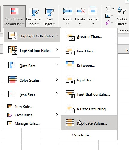Conditional Formatting Duplicate Values

4. In the Duplicate Values dialog box, choose the formatting style you want to apply to the duplicate values.
5. Click OK. Excel will highlight all the duplicate values in the selected range.

You can also use conditional formatting to highlight unique values by selecting Unique Values in the dialog box.

3.2. Using VLOOKUP for Cross-Column Comparison

VLOOKUP is a function that searches for a value in the first column of a range and returns a value from a specified column in the same row.

Syntax: =VLOOKUP(lookup_value, table_array, col_index_num, [range_lookup])

How it works:

1. lookup_value: The value you want to search for.
2. table_array: The range of cells where you want to search. The first column of this range is where the lookup_value will be searched.
3. col_index_num: The column number in the table_array from which you want to return a value.
4. [range_lookup]: Optional. TRUE for approximate match (the first column must be sorted), FALSE for exact match.

Example:

=VLOOKUP(A1, B:B, 1, FALSE)

This formula searches for the value in A1 in column B. If it finds a match, it returns the value from the same row in column B. If it doesn’t find a match, it returns #N/A. You can use the IFERROR function to handle the #N/A error.

=IFERROR(VLOOKUP(A1, B:B, 1, FALSE), "Not Found")

This formula returns “Not Found” if the value in A1 is not found in column B.

3.3. INDEX and MATCH Functions for Flexible Lookup

The INDEX and MATCH functions can be combined to perform more flexible lookups than VLOOKUP. INDEX returns a value from a specified row and column in a range, while MATCH returns the relative position of an item in a range.

Syntax:

• INDEX(array, row_num, [column_num])
• MATCH(lookup_value, lookup_array, [match_type])

How it works:

1. array: The range of cells from which you want to return a value.
2. row_num: The row number in the array from which you want to return a value.
3. [column_num]: Optional. The column number in the array from which you want to return a value.
4. lookup_value: The value you want to search for.
5. lookup_array: The range of cells where you want to search.
6. [match_type]: Optional. 0 for exact match, 1 for less than, -1 for greater than.

Example:

=INDEX(B:B, MATCH(A1, A:A, 0))

This formula searches for the value in A1 in column A and returns the corresponding value from column B in the same row.

3.4. Using Array Formulas for Complex Criteria

Array formulas allow you to perform calculations on multiple values at once, making them useful for complex comparisons.

Example:

To compare two columns and return TRUE if all values in a row are the same, you can use the following array formula:

{=AND(A1:A10=B1:B10)}

How it works:

1. Enter the formula in a cell.
2. Press Ctrl+Shift+Enter to enter it as an array formula. Excel will add curly braces {} around the formula.

This formula compares each cell in the range A1:A10 with the corresponding cell in the range B1:B10 and returns TRUE only if all the values are the same.

3.5. Power Query for Data Transformation and Comparison

Power Query is a data transformation and preparation tool in Excel that allows you to import data from various sources, clean and transform it, and load it into Excel. It can be used to compare data from different sources and identify duplicates.

Steps to compare data using Power Query:

1. Import the data into Power Query.
2. Use the Merge Queries feature to combine the data from different sources based on a common column.
3. Use the Group By feature to identify duplicate values.
4. Load the transformed data into Excel.

Power Query is particularly useful when dealing with large datasets or data from multiple sources.

4. Practical Scenarios: How to Compare Cells for Duplicates in Excel

Let’s explore some practical scenarios where comparing cells for duplicates in Excel is essential.

4.1. Comparing Customer Lists

Imagine you have two customer lists from different sources, and you want to identify customers who appear on both lists.

Steps:

1. Copy both lists into separate columns in Excel.
2. Use the COUNTIF function to check if each customer in the first list exists in the second list.
   =IF(COUNTIF(B:B, A1)>0, "Duplicate", "Unique")
3. Apply conditional formatting to highlight the duplicate customer names.

This allows you to merge the lists and avoid sending duplicate marketing materials or offers to the same customers.

4.2. Comparing Product Catalogs

If you manage a product catalog and receive updates from different suppliers, you need to ensure that the product information is consistent and accurate.

Steps:

1. Import the product catalogs into separate sheets in Excel.
2. Use VLOOKUP or INDEX/MATCH to compare the product information (e.g., name, price, description) between the catalogs.
   =IFERROR(VLOOKUP(A2,Sheet2!A:C,3,FALSE),"Not Found")
3. Use conditional formatting to highlight any discrepancies in the product information.

This helps you maintain an accurate and up-to-date product catalog.

4.3. Comparing Financial Records

In financial analysis, it’s crucial to identify duplicate transactions or entries that may indicate errors or fraud.

Steps:

1. Copy the financial records into Excel.
2. Use conditional formatting to highlight duplicate transaction amounts and dates.
3. Use the COUNTIF function to identify transactions with the same amount and date.
   =IF(COUNTIFS(A:A,A2,B:B,B2)>1,"Duplicate","")

This helps you identify and investigate potential errors or fraudulent activities.

4.4. Comparing Survey Responses

When analyzing survey responses, you may want to identify respondents who have submitted multiple responses or provided inconsistent answers.

Steps:

1. Import the survey responses into Excel.
2. Use the COUNTIF function to count the number of responses from each respondent.
   =COUNTIF(A:A,A2)
3. Use conditional formatting to highlight respondents with multiple responses.
4. Compare the answers provided by the same respondents to identify any inconsistencies.

This helps you ensure the validity and reliability of the survey data.

4.5. Comparing Inventory Lists

Maintaining an accurate inventory list is crucial for any business that manages physical products. Comparing inventory lists from different sources can help identify discrepancies and ensure that the inventory levels are accurate.

Steps:

1. Import the inventory lists into separate sheets in Excel.
2. Use VLOOKUP or INDEX/MATCH to compare the product quantities between the lists.
   =IFERROR(VLOOKUP(A2,Sheet2!A:C,3,FALSE),"Not Found")
3. Use conditional formatting to highlight any discrepancies in the product quantities.

This helps you reconcile the inventory lists and identify any shortages or overages.

5. Best Practices for Comparing Cells in Excel

To ensure accurate and efficient comparisons, follow these best practices when comparing cells in Excel.

5.1. Data Cleaning and Preparation

Before comparing cells, ensure that the data is clean and consistent. This includes:

• Removing any leading or trailing spaces.
• Standardizing the data format (e.g., dates, numbers, text).
• Correcting any typos or errors.
• Using the TRIM function to remove extra spaces: =TRIM(A1)
• Using the UPPER or LOWER function to standardize the case: =UPPER(A1) or =LOWER(A1)

5.2. Using Consistent Formulas

When comparing cells using formulas, ensure that you use consistent formulas throughout the entire range. This avoids any inconsistencies or errors in the comparison results.

5.3. Handling Errors and Missing Values

When comparing cells, you may encounter errors or missing values. Use the IFERROR function to handle these errors and provide meaningful results.

Example:

=IFERROR(VLOOKUP(A1, B:B, 1, FALSE), "Not Found")

This formula returns “Not Found” if the VLOOKUP function returns an error.

5.4. Testing and Validation

After comparing cells, test and validate the results to ensure that they are accurate. This can involve manually checking a sample of the results or using additional formulas to verify the comparison.

5.5. Documentation and Comments

Document the comparison process and add comments to the formulas to explain their purpose. This makes it easier for others to understand and maintain the spreadsheet.

• To add a comment to a cell, right-click on the cell and select Insert Comment.

5.6. Backing Up Your Data

Before making any changes to the data, back up your spreadsheet to avoid losing any important information. This ensures that you can always revert to the original data if something goes wrong.

5.7. Optimizing Performance for Large Datasets

When working with large datasets, comparing cells can be slow and resource-intensive. To optimize performance:

• Use efficient formulas and avoid unnecessary calculations.
• Use conditional formatting sparingly.
• Consider using Power Query to perform data transformations and comparisons.
• Close any unnecessary programs to free up system resources.

6. FAQs About Comparing Cells in Excel for Duplicates

Here are some frequently asked questions about comparing cells in Excel for duplicates.

6.1. How can I compare two columns in Excel and return a third column with the differences?

You can use the IF function combined with the EXACT function to compare two columns and return a third column with the differences.

Example:

=IF(EXACT(A1, B1), "", A1&" is different from "&B1)

This formula compares the values in A1 and B1. If they are the same, it returns an empty string. If they are different, it returns a string indicating the difference.

6.2. How can I compare two lists in Excel and highlight the matches?

You can use conditional formatting to highlight the matches between two lists in Excel.

Steps:

1. Select the first list.
2. Go to the Home tab, click on Conditional Formatting, and select New Rule.
3. Choose Use a formula to determine which cells to format.
4. Enter the formula =COUNTIF($B:$B, A1)>0, where A1 is the first cell in the first list and B:B is the second list.
5. Choose the formatting style you want to apply to the matches.
6. Click OK.

6.3. How can I compare multiple columns in Excel and identify the rows with the same values across all columns?

You can use the AND function to compare multiple columns and identify the rows with the same values across all columns.

Example:

=AND(A1=B1, A1=C1, A1=D1)

This formula returns TRUE if the values in A1, B1, C1, and D1 are the same, and FALSE otherwise.

6.4. How can I compare two columns in Excel and remove the duplicate rows?

You can use the Remove Duplicates feature in Excel to remove the duplicate rows.

Steps:

1. Select the range of cells you want to check for duplicates.
2. Go to the Data tab and click on Remove Duplicates.
3. In the Remove Duplicates dialog box, select the columns you want to check for duplicates.
4. Click OK.

Excel will remove the duplicate rows based on the selected columns.

6.5. How can I compare two columns in Excel and find the unique values in each column?

You can use the COUNTIF function to find the unique values in each column.

Example:

To find the unique values in column A that are not present in column B:

=IF(COUNTIF(B:B, A1)=0, A1, "")

This formula returns the value in A1 if it is not present in column B, and an empty string otherwise.

7. Conclusion: Leveraging COMPARE.EDU.VN for Data Comparison Needs

Comparing cells in Excel for duplicates is a critical task for maintaining data integrity, improving efficiency, and making informed decisions. By understanding the basic and advanced techniques, following best practices, and leveraging resources like COMPARE.EDU.VN, you can effectively compare data and ensure the accuracy of your spreadsheets.

COMPARE.EDU.VN offers a wealth of information and resources to help you master Excel and other data analysis tools. Whether you need to compare customer lists, product catalogs, financial records, or survey responses, COMPARE.EDU.VN provides comprehensive guidance and support.

Ready to take your data comparison skills to the next level? Visit COMPARE.EDU.VN today to explore our extensive collection of articles, tutorials, and tools. With COMPARE.EDU.VN, you can unlock the full potential of Excel and make data-driven decisions with confidence.

Address: 333 Comparison Plaza, Choice City, CA 90210, United States

WhatsApp: +1 (626) 555-9090

Website: compare.edu.vn