**How To Compare And Find Difference In Excel: A Detailed Guide**

Comparing and finding differences in Excel can be a time-consuming task, but with the right techniques, it can become a breeze; let COMPARE.EDU.VN show you how. This comprehensive guide explores various methods, from using simple formulas to leveraging advanced features like conditional formatting and lookup functions, empowering you to efficiently identify similarities and discrepancies in your data. Learn effective data analysis and data comparison techniques to streamline your spreadsheet tasks.

1. Why Comparing Columns in Excel is Essential

Excel is a powerful tool for data storage, organization, and analysis. One of its most useful features is the ability to compare two columns of data. This can be helpful for a variety of reasons, such as:

Identifying duplicates: Comparing two columns can help you identify duplicate entries, which can be useful for cleaning up your data and ensuring accuracy.
Finding differences: Comparing two columns can also help you find differences between them, which can be useful for tracking changes over time or identifying errors.
Validating data: Comparing two columns can help you validate data by ensuring that it is consistent across different sources.

1.1. Real-World Applications of Column Comparison

Comparing two columns in Excel is a fundamental skill with wide-ranging applications across various fields. Here are a few examples:

Finance: Comparing actual expenses against budgeted amounts to identify variances and potential overspending.
Marketing: Analyzing customer lists from different campaigns to identify overlaps and target specific segments effectively.
Sales: Comparing sales data from different periods to track performance and identify growth opportunities.
Human Resources: Validating employee data across different systems to ensure accuracy and consistency.
Inventory Management: Comparing inventory levels against sales data to identify slow-moving items and optimize stock levels.

1.2. Benefits of Efficient Column Comparison

Mastering the art of comparing columns in Excel offers several benefits:

Time Savings: Automate the comparison process and eliminate manual effort, saving valuable time and resources.
Improved Accuracy: Reduce the risk of human error associated with manual comparison, ensuring accurate results.
Data-Driven Decisions: Gain insights from data comparisons to make informed decisions and drive business outcomes.
Enhanced Productivity: Streamline data analysis workflows and improve overall productivity.
Better Data Quality: Identify and correct inconsistencies in data, leading to improved data quality and reliability.

2. Different Methods to Compare Columns in Excel

Excel offers several methods for comparing two columns, each with its own strengths and weaknesses. The best method for you will depend on the specific task you are trying to accomplish and the size and complexity of your data.

Here are some of the most common methods:

Equals Operator (=): This simple operator compares two cells and returns TRUE if they are equal and FALSE if they are not.
IF Function: This function allows you to perform a logical test and return different values based on the result.
EXACT Function: This function compares two text strings and returns TRUE only if they are exactly the same, including case.
Conditional Formatting: This feature allows you to highlight cells that meet certain criteria.
LOOKUP Functions (VLOOKUP, HLOOKUP, XLOOKUP): These functions allow you to search for a value in one column and return a corresponding value from another column.

2.1. Factors to Consider When Choosing a Method

When selecting a method for comparing columns, consider the following factors:

Data Type: Are you comparing numbers, text strings, dates, or other data types?
Case Sensitivity: Do you need to consider case when comparing text strings?
Complexity: How complex is the comparison you need to perform?
Data Size: How large is the dataset you are working with?
Desired Output: What type of output do you need? Do you need to identify matching values, differing values, or both?

2.2. Overview of the Most Common Techniques

Let’s take a closer look at some of the most common techniques for comparing columns in Excel:

Technique	Description	Best Use Case
Equals Operator (=)	Compares two cells and returns TRUE or FALSE.	Simple comparisons of numbers or text strings.
IF Function	Performs a logical test and returns different values based on the result.	More complex comparisons with multiple conditions.
EXACT Function	Compares two text strings and returns TRUE only if they are exactly the same, including case.	Case-sensitive comparisons of text strings.
Conditional Formatting	Highlights cells that meet certain criteria.	Visualizing differences and duplicates.
LOOKUP Functions	Searches for a value in one column and returns a corresponding value from another column.	Finding related data in different columns.

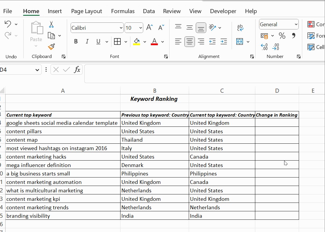
3. Comparing Two Columns Using the Equals Operator

The equals operator (=) is the simplest way to compare two cells in Excel. It returns TRUE if the values in the two cells are equal and FALSE if they are not.

3.1. Step-by-Step Guide to Using the Equals Operator

Here’s how to use the equals operator to compare two columns:

Select a cell where you want to display the result of the comparison.
Enter the formula =column1=column2, where column1 and column2 are the cell references of the two cells you want to compare. For example, if you want to compare cell B4 with cell C4, you would enter the formula =B4=C4.
Press Enter. The formula will return TRUE if the values in the two cells are equal and FALSE if they are not.
Drag the fill handle (the small square at the bottom right corner of the cell) down to apply the formula to the rest of the rows in your data.

3.2. Advantages and Limitations of This Method

Advantages:

Simple and easy to use.
Fast for small datasets.

Limitations:

Only works for simple comparisons.
Cannot handle case-sensitive comparisons.
Does not provide any information about the differences between the two cells if they are not equal.

3.3. Examples of How to Apply the Equals Operator

Here are a few examples of how to apply the equals operator:

Comparing two lists of names: You can use the equals operator to compare two lists of names to identify any duplicates or differences.
Comparing two sets of numbers: You can use the equals operator to compare two sets of numbers to identify any discrepancies.
Comparing two dates: You can use the equals operator to compare two dates to see if they are the same.

4. Comparing Two Columns Using the IF Condition

The IF function is a more powerful way to compare two columns in Excel. It allows you to perform a logical test and return different values based on the result.

4.1. Explaining the Syntax and Logic of the IF Function

The syntax of the IF function is as follows:

=IF(logical_test, value_if_true, value_if_false)

logical_test: This is the condition that you want to test. It can be any expression that evaluates to TRUE or FALSE.
value_if_true: This is the value that will be returned if the logical_test is TRUE.
value_if_false: This is the value that will be returned if the logical_test is FALSE.

4.2. Using IF to Display “Match” or “Not Match”

Here’s how to use the IF function to display “Match” or “Not Match” when comparing two columns:

Select a cell where you want to display the result of the comparison.
Enter the formula =IF(column1=column2,"Match","Not Match"), where column1 and column2 are the cell references of the two cells you want to compare. For example, if you want to compare cell B4 with cell C4, you would enter the formula =IF(B4=C4,"Match","Not Match").
Press Enter. The formula will return “Match” if the values in the two cells are equal and “Not Match” if they are not.
Drag the fill handle down to apply the formula to the rest of the rows in your data.

4.3. Identifying Mismatched Values with IF and the Not Equal To Operator (<>)

To compare two columns in Excel for differences, replace the equals sign with the non-equality sign (<>). The formula is =IF(A2<>B2,”Match”,”Not a Match “).

This formula will return “Match” if the values in the two cells are different and “Not a Match” if they are the same.

5. Comparing Two Columns Using the EXACT() Function

The EXACT() function compares two text strings and returns TRUE only if they are exactly the same, including case. This is useful when you need to perform a case-sensitive comparison.

5.1. Understanding the EXACT() Function’s Case-Sensitive Nature

Unlike the equals operator and the IF function, the EXACT() function is case-sensitive. This means that it will treat “Apple” and “apple” as different values.

5.2. Combining EXACT() with IF() for Case-Sensitive Comparisons

Here’s how to combine the EXACT() function with the IF() function for case-sensitive comparisons:

Select a cell where you want to display the result of the comparison.
Enter the formula =IF(EXACT(column1,column2),"Match","Not Match"), where column1 and column2 are the cell references of the two cells you want to compare. For example, if you want to compare cell B4 with cell C4, you would enter the formula =IF(EXACT(B4,C4),"Match","Not Match").
Press Enter. The formula will return “Match” if the values in the two cells are exactly the same, including case, and “Not Match” if they are not.
Drag the fill handle down to apply the formula to the rest of the rows in your data.

5.3. Scenarios Where EXACT() Is Particularly Useful

The EXACT() function is particularly useful in scenarios where case sensitivity is important, such as:

Comparing usernames and passwords: Usernames and passwords are typically case-sensitive, so you would need to use the EXACT() function to compare them.
Comparing product codes: Product codes may also be case-sensitive, so you would need to use the EXACT() function to compare them.
Comparing scientific data: Scientific data may contain case-sensitive symbols or abbreviations, so you would need to use the EXACT() function to compare them.

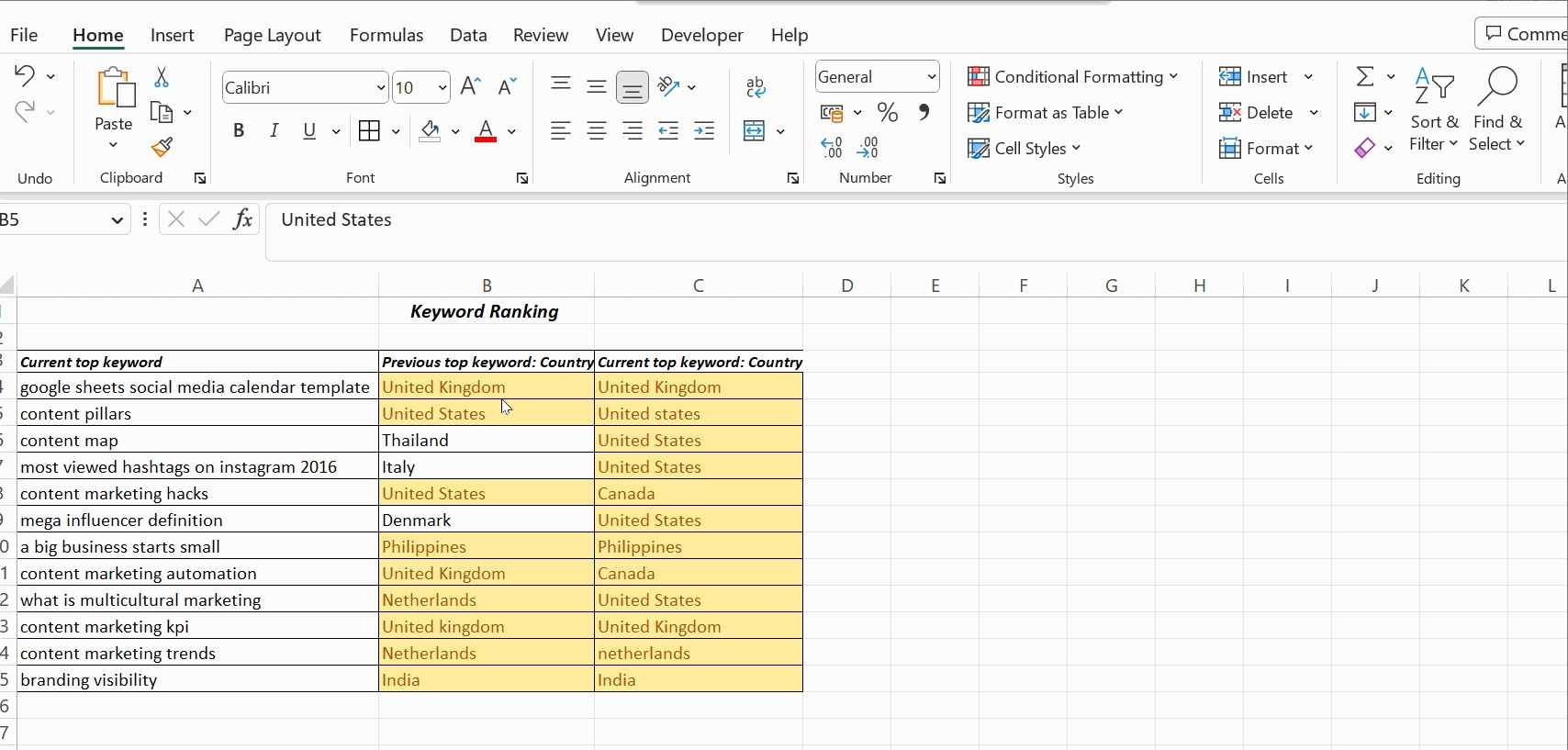
6. Comparing Two Columns Using Conditional Formatting

Conditional formatting is a powerful feature that allows you to highlight cells that meet certain criteria. This can be useful for visually identifying differences and duplicates in two columns.

6.1. Highlighting Duplicate Values in Two Columns

Here’s how to use conditional formatting to highlight duplicate values in two columns:

Select the two columns you want to compare.
Click on the “Home” tab in the Excel ribbon.
Click on “Conditional Formatting” in the “Styles” group.
Select “Highlight Cells Rules” and then “Duplicate Values”.
Choose the formatting you want to apply to the duplicate values. You can choose to fill the cells with a specific color, change the font color, or add a border.
Click “OK”. Excel will highlight all the duplicate values in the two columns.

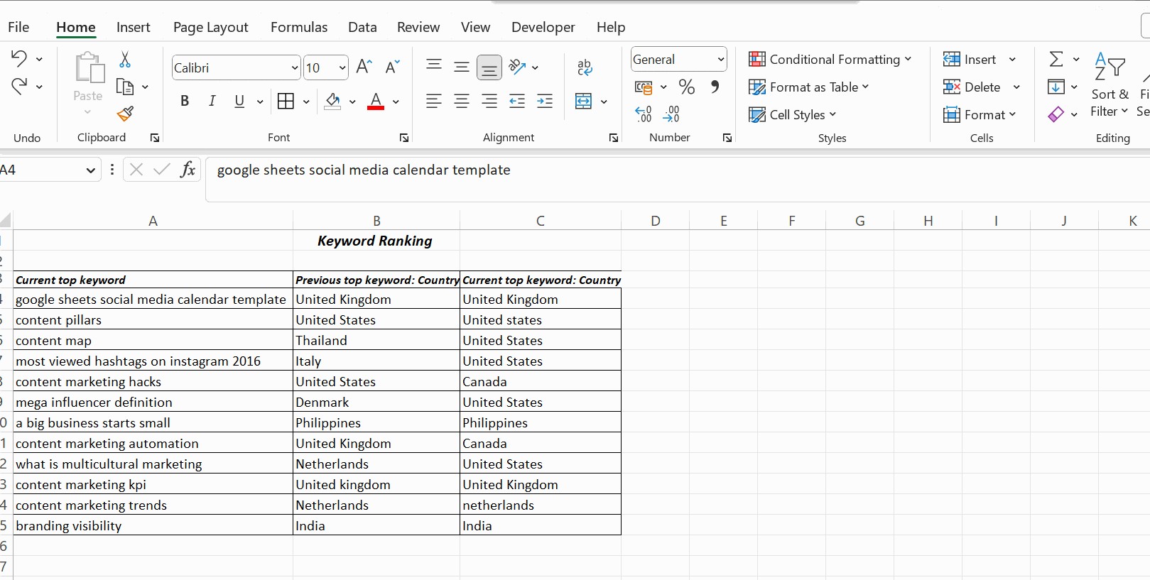
6.2. Highlighting Unique Values in Two Columns

Here’s how to use conditional formatting to highlight unique values in two columns:

Select the two columns you want to compare.
Click on the “Home” tab in the Excel ribbon.
Click on “Conditional Formatting” in the “Styles” group.
Select “Highlight Cells Rules” and then “Duplicate Values”.
In the “Duplicate Values” dialog box, select “Unique” from the drop-down menu.
Choose the formatting you want to apply to the unique values.
Click “OK”. Excel will highlight all the unique values in the two columns.

6.3. Customizing Conditional Formatting Rules for Specific Needs

You can customize conditional formatting rules to meet your specific needs. For example, you can create a rule that highlights cells that are greater than, less than, or equal to a certain value. You can also create rules that highlight cells that contain specific text or dates.

To customize conditional formatting rules, select the columns you want to format, click on “Conditional Formatting” in the “Styles” group, and then select “New Rule”. In the “New Formatting Rule” dialog box, you can choose the type of rule you want to create and specify the criteria for the rule.

7. Using Lookup Functions to Compare Two Columns

Lookup functions are powerful tools that allow you to search for a value in one column and return a corresponding value from another column. This can be useful for comparing two columns and identifying differences or matches.

7.1. Introduction to VLOOKUP, HLOOKUP, and XLOOKUP

Excel offers several lookup functions, including:

VLOOKUP: This function searches for a value in the first column of a range and returns a corresponding value from another column in the same row.
HLOOKUP: This function searches for a value in the first row of a range and returns a corresponding value from another row in the same column.
XLOOKUP: This function is a more versatile lookup function that can search for a value in any column or row and return a corresponding value from any other column or row.

7.2. How VLOOKUP Can Help in Column Comparison

VLOOKUP can be used to compare two columns by searching for values in one column and returning corresponding values from the other column. This can help you identify:

Matching values: If VLOOKUP finds a match for a value in the first column, it will return the corresponding value from the second column.
Missing values: If VLOOKUP does not find a match for a value in the first column, it will return an error.
Different values: If VLOOKUP finds a match for a value in the first column but the corresponding value in the second column is different, it will return the different value.

7.3. Practical Examples of Using VLOOKUP for Data Matching

Here’s a practical example of how to use VLOOKUP for data matching:

Suppose you have two columns of data:

Column A (Product ID)	Column B (Product Name)
1001	Apple
1002	Banana
1003	Orange

Column C (Product ID)	Column D (Price)
1001	1.00
1003	1.25
1004	1.50

You can use VLOOKUP to find the price of each product in Column A by searching for the Product ID in Column C and returning the corresponding Price from Column D.

The formula would be: =VLOOKUP(A1,C:D,2,FALSE)

This formula will search for the value in cell A1 (Product ID) in Column C and return the corresponding value from Column D (Price). The FALSE argument tells VLOOKUP to find an exact match.

8. Advanced Techniques for Complex Comparisons

For more complex comparisons, you may need to use more advanced techniques, such as:

Combining multiple functions: You can combine multiple functions to perform more complex comparisons. For example, you can combine the IF function with the AND or OR functions to test multiple conditions.
Using array formulas: Array formulas allow you to perform calculations on multiple cells at once. This can be useful for comparing two columns and identifying differences or matches across multiple rows.
Using VBA macros: VBA macros allow you to automate complex tasks in Excel. This can be useful for comparing two columns and performing custom calculations or formatting.

8.1. Combining Multiple Functions for Sophisticated Logic

Combining multiple functions allows you to create more sophisticated logic for your comparisons. For example, you can use the AND function to test multiple conditions and return a value only if all of the conditions are TRUE. You can also use the OR function to test multiple conditions and return a value if any of the conditions are TRUE.

8.2. Utilizing Array Formulas for Multi-Cell Comparisons

Array formulas allow you to perform calculations on multiple cells at once. This can be useful for comparing two columns and identifying differences or matches across multiple rows. To enter an array formula, you must press Ctrl+Shift+Enter.

8.3. Automating Comparisons with VBA Macros

VBA macros allow you to automate complex tasks in Excel. This can be useful for comparing two columns and performing custom calculations or formatting. To create a VBA macro, you must open the Visual Basic Editor (VBE) by pressing Alt+F11.

9. Tips and Tricks for Efficient Column Comparison

Here are some tips and tricks for efficient column comparison:

Sort your data: Sorting your data can make it easier to identify duplicates and differences.
Use filters: Filters can help you narrow down your data and focus on specific values.
Use helper columns: Helper columns can be used to perform intermediate calculations or store temporary results.
Use keyboard shortcuts: Keyboard shortcuts can help you speed up your work.
Test your formulas: Always test your formulas to make sure they are working correctly.

9.1. Sorting and Filtering Data for Easier Analysis

Sorting and filtering data can make it easier to identify duplicates and differences. For example, you can sort your data by one of the columns you are comparing and then filter the data to show only the rows where the values in the two columns are different.

9.2. Using Helper Columns to Simplify Complex Formulas

Helper columns can be used to perform intermediate calculations or store temporary results. This can make your formulas easier to read and understand. For example, you can use a helper column to calculate the difference between two values and then use another formula to compare the difference to a threshold.

9.3. Keyboard Shortcuts to Speed Up the Comparison Process

Keyboard shortcuts can help you speed up your work. Here are some useful keyboard shortcuts for comparing columns in Excel:

Ctrl+C: Copy
Ctrl+V: Paste
Ctrl+X: Cut
Ctrl+Z: Undo
Ctrl+Y: Redo
Ctrl+A: Select All
Ctrl+F: Find
Ctrl+H: Replace
F2: Edit Cell
F4: Repeat Last Action

10. Common Mistakes to Avoid When Comparing Columns

Here are some common mistakes to avoid when comparing columns:

Not considering case sensitivity: The equals operator and the IF function are not case-sensitive. If you need to perform a case-sensitive comparison, you must use the EXACT() function.
Not handling errors: If your formulas encounter errors, they may return incorrect results. Make sure to handle errors in your formulas using the IFERROR() function.
Not testing your formulas: Always test your formulas to make sure they are working correctly.
Not using the right tool for the job: Excel offers several different methods for comparing columns. Make sure to choose the right method for the specific task you are trying to accomplish.
Comparing unmatched data types: Be sure that the columns you are comparing are of the same data type

10.1. Ignoring Case Sensitivity When It Matters

As mentioned earlier, the equals operator and the IF function are not case-sensitive. If you need to perform a case-sensitive comparison, you must use the EXACT() function.

10.2. Overlooking Data Type Differences

Excel stores data in various formats such as Text, Number, Currency, Date, etc. To get an accurate result, make sure the column values you are comparing have the same data type.

10.3. Not Handling Errors in Formulas

If your formulas encounter errors, they may return incorrect results. Make sure to handle errors in your formulas using the IFERROR() function. The IFERROR() function allows you to specify a value to return if a formula returns an error.

11. FAQ: Answering Common Questions About Column Comparison

Here are some frequently asked questions about column comparison in Excel:

11.1. How Do I Compare Two Columns in Excel?

There are several methods, including using the equals operator (=), IF function, EXACT function, conditional formatting, and lookup functions. The best method depends on your specific needs.

11.2. How Can I Highlight Differences Between Two Columns?

You can use conditional formatting to highlight differences between two columns. Select the columns you want to compare, click on “Conditional Formatting” in the “Styles” group, and then select “New Rule”. In the “New Formatting Rule” dialog box, you can choose the type of rule you want to create and specify the criteria for the rule.

11.3. How Do I Find Duplicate Values in Two Columns?

You can use conditional formatting to find duplicate values in two columns. Select the columns you want to compare, click on “Conditional Formatting” in the “Styles” group, and then select “Highlight Cells Rules” and then “Duplicate Values”.

11.4. Can I Compare More Than Two Columns at Once?

Yes, you can compare more than two columns at once by combining multiple functions or using array formulas.

11.5. How Do I Compare Two Columns With Different Lengths?

You can use the IFERROR() function to handle errors that occur when comparing two columns with different lengths. The IFERROR() function allows you to specify a value to return if a formula returns an error.

11.6. How Do I Compare Two Columns Ignoring Case?

Use the UPPER() or LOWER() functions in conjunction with the IF() function to convert both columns to the same case before comparing. For example: =IF(UPPER(A1)=UPPER(B1), "Match", "No Match").

11.7. What Is The Best Way To Compare Two Columns With Dates?

Ensure both columns are formatted as dates. Then, use the IF() function to compare them directly: =IF(A1=B1, "Match", "No Match").

11.8. How Do I Find The Differences In Two Columns And List Them?

Use a combination of IF(), ISERROR(), and VLOOKUP() to identify values in one column that are not in the other. Then, list these differences in a separate column.

11.9. How Can I Compare Two Columns And Count The Matches?

Use the COUNTIF() function. For example, to count how many values in column A match values in column B, use: =COUNTIF(B:B, A1). Drag the formula down column A, then sum the resulting column.

11.10. Is There A Way To Highlight Entire Rows Based On A Comparison?

Yes, use conditional formatting with a formula. Create a new rule that uses a formula to determine which cells to format. For example, to highlight the entire row if A1 and B1 do not match, use the formula =$A1<>$B1 and apply it to the range of your data.

12. Conclusion: Mastering Column Comparison in Excel

Comparing columns in Excel is a fundamental skill for data analysis. By mastering the techniques described in this guide, you can efficiently identify similarities, differences, and duplicates in your data, enabling you to make informed decisions and improve data quality.

12.1. Recap of Key Methods and Their Applications

Equals Operator (=): Simple comparisons of numbers or text strings.
IF Function: More complex comparisons with multiple conditions.
EXACT Function: Case-sensitive comparisons of text strings.
Conditional Formatting: Visualizing differences and duplicates.
LOOKUP Functions: Finding related data in different columns.

12.2. Encouragement to Explore and Practice Different Techniques

Excel is a powerful tool with a wide range of features. Don’t be afraid to experiment with different techniques and find the methods that work best for you. The more you practice, the more proficient you will become at comparing columns in Excel.

12.3. Final Thoughts on the Power of Data Comparison for Decision Making

Data comparison is a critical skill for anyone who works with data. By mastering the art of comparing columns in Excel, you can unlock the power of your data and make informed decisions that drive business outcomes.

Ready to take your Excel skills to the next level? Visit COMPARE.EDU.VN to discover more in-depth tutorials, practical examples, and expert tips to help you master data analysis and make data-driven decisions. Your journey to Excel mastery starts here!

Contact us:

Address: 333 Comparison Plaza, Choice City, CA 90210, United States

Whatsapp: +1 (626) 555-9090

Website: compare.edu.vn