How Do You Compare Two Columns In Excel For Differences? Comparing two columns in Excel to identify differences is a common task that can be efficiently accomplished using various methods. At COMPARE.EDU.VN, we provide comprehensive guides and tools to help you master this skill, enabling you to streamline data analysis and make informed decisions. Discover how to compare data, identify mismatches, and highlight discrepancies using Excel’s powerful features.
1. Why Comparing Two Columns in Excel is Essential
Excel is a powerful tool for data storage, manipulation, and analysis. Comparing two columns within Excel is essential for data analysts and anyone who needs to identify differences, inconsistencies, or matches within their datasets. This process can save time and improve accuracy compared to manual comparisons.
1.1. Data Validation and Cleaning
Comparing columns helps ensure data integrity by identifying errors, inconsistencies, and duplicates. This is crucial for maintaining accurate records. According to a study by MIT, poor data quality costs organizations an average of 15% to 25% of their revenue.
1.2. Identifying Changes and Updates
When dealing with updated datasets, comparing columns helps pinpoint new entries, modifications, or deletions, ensuring you’re always working with the most current information.
1.3. Reconciliation of Data
In accounting and finance, comparing columns ensures that financial records match, helping to prevent discrepancies and fraud.
1.4. Data Analysis and Reporting
Identifying differences and similarities between columns can provide valuable insights for data analysis and reporting, helping to inform decision-making processes.
2. Methods for Comparing Two Columns in Excel
There are several methods to compare two columns in Excel, each with its own strengths and applications. These include using the equals operator, IF condition, EXACT function, conditional formatting, and lookup functions.
2.1. Using the Equals Operator
The equals operator (=) is a basic yet effective method for comparing two columns row by row. This method returns TRUE if the values in the compared columns are the same and FALSE if they differ.
2.1.1. Formula Implementation
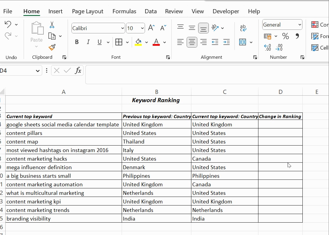
To use the equals operator, enter the formula =column1=column2 in a cell next to the rows you want to compare. For example, if you want to compare column B and column C, starting from row 4, you would enter =B4=C4 in cell D4.
2.1.2. Practical Application
Drag the formula down to apply it to all the rows in your dataset. The result will be a column of TRUE and FALSE values, indicating whether the corresponding rows match or not.
2.2. Comparing with the IF Condition
The IF condition allows you to return custom messages like “Match” or “Not Match” instead of TRUE or FALSE. This can make the results more readable and easier to interpret.
2.2.1. Basic IF Condition
The formula =IF(B4=C4,”Yes”,” “) returns “Yes” if the values in columns B and C match, and leaves the cell blank if they don’t.
2.2.2. Identifying Mismatches
To specifically identify mismatches, use the formula =IF(B4=C4,”Yes”,”No”). This returns “Yes” for matching values and “No” for mismatches.
2.2.3. Comparing for Differences
To compare two columns for differences, use the non-equality sign (<>). The formula =IF(A2<>B2,”Match”,”Not a Match”) returns “Match” if the values in columns A and B are different, and “Not a Match” if they are the same.
2.3. Using the EXACT() Function
The EXACT() function is case-sensitive, ensuring that only identical text strings are considered a match. This is useful when capitalization matters.
2.3.1. Syntax and Usage
The syntax for the EXACT() function is =EXACT(text1,text2). It takes two arguments, text1 and text2, and returns TRUE if they are exactly the same, including capitalization.
2.3.2. Combining with IF()
To use EXACT() with the IF condition, use the formula =IF(EXACT(B4,C4), “Match”, “Mismatched”). This returns “Match” only if the values in columns B and C are identical, including capitalization, and “Mismatched” otherwise.
2.3.3. Case Sensitivity
The EXACT() function is particularly useful when you need to differentiate between entries like “Netherlands” and “netherlands.”
2.4. Conditional Formatting
Conditional formatting allows you to highlight unique or duplicate values directly in the columns, providing a visual representation of the differences.
2.4.1. Highlighting Duplicate Values
To highlight duplicate values, select the columns you want to compare, then go to Home → Styles → Conditional Formatting → Highlight Cell Rules → Duplicate Values.
2.4.2. Customizing Formatting
In the dialog box, choose “Duplicate” from the drop-down menu. You can then customize the formatting to fill the cells with a specific color, change the text color, or modify the cell border.
2.4.3. Highlighting Unique Values
To highlight unique values, follow the same steps as above, but choose “Unique” from the drop-down menu instead of “Duplicate.”
2.4.4. Clearing Formatting Rules
To clear the formatting you’ve applied, go to Conditional Formatting → Clear Rules → Clear Rules from Selected Cells.
2.4.5. Visual Comparison
Conditional formatting is ideal when you want a quick visual comparison without adding a third column to display results.
2.5. Using Lookup Functions
Lookup functions like VLOOKUP, HLOOKUP, and XLOOKUP can be used to compare two columns in Excel for differences by searching for values in one column and returning corresponding values from another.
2.5.1. VLOOKUP Function
The VLOOKUP function searches for a value in the first column of a range and returns a value in the same row from a column you specify. The syntax is =VLOOKUP(lookup_value, table_array, col_index_num, [range_lookup]).
2.5.2. Applying VLOOKUP for Comparison
For example, if column A contains a list of keywords and column B contains parent keywords, you can use VLOOKUP to find the matching parent keyword for each keyword in column A. The formula would be =VLOOKUP(A4, $B$4:$B$15, 1, 0).
2.5.3. Absolute References
The $ symbol before the cell reference (e.g., $B$4:$B$15) is called an absolute reference, which ensures that the range does not change when you drag the formula down.
2.5.4. Arguments of VLOOKUP
- lookup_value: The value to search for (e.g., A4).
- table_array: The range to search in (e.g., $B$4:$B$15).
- col_index_num: The column number in the range from which to return a value (1 in this case).
- range_lookup: A logical value that specifies whether to find an exact match (0) or an approximate match (1).
3. Step-by-Step Guide to Comparing Two Columns in Excel
To effectively compare two columns in Excel, follow these steps:
3.1. Prepare Your Data
Ensure that your data is organized and cleaned. Remove any unnecessary characters or spaces that might affect the comparison.
3.2. Choose Your Method
Select the method that best suits your needs. For simple comparisons, the equals operator or IF condition might suffice. For case-sensitive comparisons, use the EXACT() function. For visual comparisons, use conditional formatting. For more complex comparisons, use lookup functions.
3.3. Implement the Formula or Formatting
Enter the appropriate formula in a new column or apply conditional formatting to the columns you want to compare.
3.4. Analyze the Results
Review the results and take appropriate action. For example, if you find mismatches, investigate the cause and correct the data.
4. Advanced Techniques for Column Comparison
For more complex scenarios, consider using advanced techniques such as array formulas, custom functions, and VBA scripts.
4.1. Array Formulas
Array formulas can perform multiple calculations at once, making them useful for comparing entire columns without dragging formulas down.
4.1.1. Syntax and Usage
To enter an array formula, type the formula and press Ctrl+Shift+Enter instead of just Enter. Excel will automatically add curly braces {} around the formula.
4.1.2. Example
For instance, to compare two columns and return an array of TRUE/FALSE values, you can use a formula like {=A1:A10=B1:B10}.
4.2. Custom Functions
Custom functions (also known as User-Defined Functions or UDFs) allow you to create your own functions in VBA to perform specific tasks.
4.2.1. Creating a Custom Function
To create a custom function, open the VBA editor (Alt + F11), insert a new module (Insert → Module), and write your function.
4.2.2. Example
For example, you can create a function that compares two cells and returns “Match” or “Mismatch”:
Function CompareCells(cell1 As Range, cell2 As Range) As String
    If cell1.Value = cell2.Value Then
        CompareCells = "Match"
    Else
        CompareCells = "Mismatch"
    End If
End Function
4.2.3. Using the Custom Function
You can then use this function in your worksheet like any other Excel function: =CompareCells(A1, B1).
4.3. VBA Scripts
VBA scripts can automate complex comparison tasks, such as highlighting all differences between two columns or creating a summary report.
4.3.1. Writing a VBA Script
To write a VBA script, open the VBA editor (Alt + F11), insert a new module (Insert → Module), and write your script.
4.3.2. Example
For instance, you can write a script that highlights all the cells in column A that are different from the corresponding cells in column B:
Sub HighlightDifferences()
    Dim i As Long
    Dim lastRow As Long

    lastRow = Cells(Rows.Count, "A").End(xlUp).Row

    For i = 1 To lastRow
        If Cells(i, "A").Value <> Cells(i, "B").Value Then
            Cells(i, "A").Interior.Color = RGB(255, 0, 0) 'Red
        End If
    Next i
End Sub
4.3.3. Running the VBA Script
You can run the script by pressing F5 in the VBA editor or by assigning it to a button on your worksheet.
5. Use Cases for Comparing Two Columns in Excel
Comparing two columns in Excel is useful in various scenarios across different industries.
5.1. Finance and Accounting
In finance and accounting, comparing columns is crucial for reconciling bank statements, identifying discrepancies in financial records, and ensuring compliance.
5.2. Sales and Marketing
In sales and marketing, comparing columns can help identify leads, track campaign performance, and analyze customer data.
5.3. Human Resources
In human resources, comparing columns can help manage employee records, track training progress, and ensure compliance with labor laws.
5.4. Inventory Management
In inventory management, comparing columns can help track stock levels, identify discrepancies between physical inventory and recorded data, and optimize supply chain operations.
5.5. Education
In education, comparing columns can help manage student records, track academic progress, and analyze exam results. According to a report by the U.S. Department of Education, data-driven decision-making can significantly improve student outcomes.
6. Common Mistakes to Avoid When Comparing Columns in Excel
To ensure accurate comparisons, avoid these common mistakes:
6.1. Ignoring Case Sensitivity
Be mindful of case sensitivity when comparing text values. Use the EXACT() function when capitalization matters.
6.2. Overlooking Hidden Characters
Hidden characters such as spaces or non-printing characters can affect comparison results. Use the TRIM() and CLEAN() functions to remove these characters.
6.3. Not Using Absolute References
When using lookup functions, use absolute references ($) to prevent ranges from changing when you drag formulas down.
6.4. Not Validating Data
Ensure that your data is validated and cleaned before comparing columns. This includes checking for errors, inconsistencies, and duplicates.
6.5. Not Understanding Data Types
Be aware of data types (e.g., numbers, text, dates) and ensure that you are comparing values of the same type. Use the VALUE(), TEXT(), and DATE() functions to convert values if necessary.
7. Optimizing Your Excel Skills with COMPARE.EDU.VN
At COMPARE.EDU.VN, we understand the importance of efficient data analysis and decision-making. Our platform offers a wealth of resources to help you master Excel and other tools.
7.1. Comprehensive Guides and Tutorials
We provide step-by-step guides and tutorials on various Excel functions and features, including column comparison techniques.
7.2. Expert Advice and Tips
Our team of experts shares valuable insights and tips to help you optimize your Excel skills and improve your data analysis capabilities.
7.3. Interactive Tools and Templates
We offer interactive tools and templates to help you practice and apply what you’ve learned, making it easier to master Excel.
7.4. Community Support
Join our community of users to ask questions, share tips, and learn from others.
8. Real-World Examples of Column Comparison
Let’s explore some real-world examples of how column comparison can be used in different industries.
8.1. Example 1: Comparing Sales Data
A sales manager wants to compare sales data from two different quarters to identify top-performing products and areas for improvement.
8.1.1. Data Setup
Column A: Product Names (Quarter 1)
Column B: Sales Revenue (Quarter 1)
Column C: Product Names (Quarter 2)
Column D: Sales Revenue (Quarter 2)
8.1.2. Steps
- Use the IF condition to compare product names in Quarter 1 and Quarter 2: =IF(A2=C2, “Match”, “New Product”)
- Use VLOOKUP to find the sales revenue for matching products: =VLOOKUP(A2, C:D, 2, FALSE)
- Calculate the difference in sales revenue: =B2-VLOOKUP(A2, C:D, 2, FALSE)
- Use conditional formatting to highlight significant changes in sales revenue.
8.1.3. Benefits
- Identifies new products introduced in Quarter 2.
- Tracks changes in sales revenue for existing products.
- Highlights top-performing and underperforming products.
8.2. Example 2: Comparing Inventory Data
An inventory manager wants to compare inventory data from two different systems to identify discrepancies and ensure accurate stock levels.
8.2.1. Data Setup
Column A: Product Codes (System 1)
Column B: Quantity (System 1)
Column C: Product Codes (System 2)
Column D: Quantity (System 2)
8.2.2. Steps
- Use the IF condition to compare product codes in System 1 and System 2: =IF(A2=C2, “Match”, “New Product”)
- Use VLOOKUP to find the quantity for matching products: =VLOOKUP(A2, C:D, 2, FALSE)
- Calculate the difference in quantity: =B2-VLOOKUP(A2, C:D, 2, FALSE)
- Use conditional formatting to highlight significant discrepancies in quantity.
8.2.3. Benefits
- Identifies new products in System 2.
- Tracks discrepancies in quantity for existing products.
- Highlights products with significant stock level differences.
9. Conclusion: Mastering Column Comparison in Excel
Comparing two columns in Excel is a fundamental skill that can significantly improve your data analysis capabilities. By mastering the various methods and techniques discussed in this guide, you can streamline your workflow, improve accuracy, and make more informed decisions.
Remember to leverage the resources available at COMPARE.EDU.VN to further enhance your Excel skills and stay ahead of the curve. Our comprehensive guides, expert advice, and interactive tools are designed to help you excel in data analysis and achieve your goals.
10. Frequently Asked Questions
10.1. How do you compare two columns in Excel to find differences?
You can compare two columns in Excel for differences by using the equals operator (=), IF condition, EXACT() function, conditional formatting, or lookup functions like VLOOKUP. The best method depends on your specific needs and the type of data you are comparing.
10.2. How can I compare two columns in Excel ignoring case?
To compare two columns in Excel ignoring case, you can use the UPPER() or LOWER() functions to convert the text to the same case before comparing them. For example, you can use the formula =IF(UPPER(A1)=UPPER(B1), “Match”, “Mismatch”).
10.3. What is the best way to highlight differences between two columns in Excel?
The best way to highlight differences between two columns in Excel is to use conditional formatting. Select the columns you want to compare, go to Home → Styles → Conditional Formatting → Highlight Cell Rules, and choose the appropriate rule (e.g., Duplicate Values, Unique Values, or More Rules).
10.4. How do I compare three or more columns in Excel?
To find matches in all cells when the table has three or more columns, use an IF() with AND statement. The formula is =IF(AND(A2=B2, A2=C2), “Full match”, “”). To find matches in any two cells in the same row, use =IF(OR(A2=B2, B2=C2, A2=C2), “Match”, “”).
10.5. Can I use VBA to compare two columns in Excel?
Yes, you can use VBA to compare two columns in Excel. VBA scripts can automate complex comparison tasks, such as highlighting all differences between two columns or creating a summary report. An example script is provided in section 4.3.2.
10.6. How do I compare two columns in Excel for partial matches?
To compare two columns in Excel for partial matches, you can use the SEARCH() or FIND() functions. These functions return the starting position of one text string inside another. For example, you can use the formula =IF(ISNUMBER(SEARCH(A1, B1)), “Partial Match”, “No Match”).
10.7. What is the difference between VLOOKUP and HLOOKUP?
VLOOKUP (Vertical Lookup) searches for a value in the first column of a range and returns a value in the same row from a column you specify. HLOOKUP (Horizontal Lookup) searches for a value in the first row of a range and returns a value in the same column from a row you specify.
10.8. How do I handle errors when comparing columns in Excel?
To handle errors when comparing columns in Excel, you can use the IFERROR() function. This function allows you to return a custom value if a formula results in an error. For example, you can use the formula =IFERROR(VLOOKUP(A1, B:C, 2, FALSE), “Not Found”) to return “Not Found” if VLOOKUP results in an error.
10.9. How can I remove duplicate values before comparing columns in Excel?
You can remove duplicate values before comparing columns in Excel by using the “Remove Duplicates” feature. Select the columns you want to clean, go to Data → Data Tools → Remove Duplicates, and specify the columns to check for duplicates.
10.10. How do I compare two columns with different lengths in Excel?
To compare two columns with different lengths in Excel, you can use the IF condition with ISBLANK function. For example, you can use the formula =IF(ISBLANK(A1), “”, IF(A1=B1, “Match”, “Mismatch”)) to compare only the rows where column A is not blank.
Are you ready to streamline your data analysis and make informed decisions? Visit compare.edu.vn today to discover more comprehensive guides and tools. Our platform offers a wealth of resources to help you master Excel and other tools, ensuring you stay ahead in your professional endeavors. Don’t miss out on the opportunity to enhance your skills and improve your data analysis capabilities. Contact us at 333 Comparison Plaza, Choice City, CA 90210, United States. Whatsapp: +1 (626) 555-9090.