How to Compare Three Columns in Excel Using VLOOKUP

How To Compare Three Columns In Excel Using Vlookup? COMPARE.EDU.VN offers a streamlined solution for individuals aiming to efficiently compare data across multiple columns in Excel. By mastering the VLOOKUP function and related strategies, you can quickly identify matching values, differences, and unique entries, leading to better data analysis and informed decision-making. Leverage the power of Excel for comparative analysis and data validation.

Table of Contents

1. Understanding the Basics of VLOOKUP

1.1 What is VLOOKUP?
1.2 VLOOKUP Syntax
1.3 Limitations of VLOOKUP

2. Extending VLOOKUP to Multiple Columns

2.1 The Logic Behind Multiple Column Lookup
2.2 VLOOKUP Syntax for Multiple Columns
2.3 Practical Examples

3. Comparing Three Columns Using VLOOKUP

3.1 The Nested VLOOKUP Approach
3.2 Step-by-Step Guide to Implementing Nested VLOOKUP
3.3 Handling Errors and Blank Cells

4. Alternative Methods for Comparing Columns

4.1 Using the MATCH Function
4.2 Combining INDEX and MATCH for Flexibility
4.3 Conditional Formatting for Visual Comparison

5. Advanced Techniques and Considerations

5.1 Using Array Formulas for Complex Comparisons
5.2 Handling Large Datasets
5.3 Performance Optimization Tips

6. Real-World Applications

6.1 Inventory Management
6.2 Financial Analysis
6.3 Customer Data Comparison

7. Troubleshooting Common Issues

7.1 #N/A Errors
7.2 Incorrect Matches
7.3 Performance Bottlenecks

8. Automating Data Import to Excel

8.1 Using Power Query
8.2 Third-Party Tools for Data Integration

9. Excel Online vs. Desktop Version

9.1 Differences in Functionality
9.2 Cloud Collaboration Benefits

10. Frequently Asked Questions (FAQ)

11. Conclusion

1. Understanding the Basics of VLOOKUP

Before diving into comparing three columns, it’s essential to grasp the fundamentals of the VLOOKUP function. This section will cover the basics, syntax, and inherent limitations.

1.1 What is VLOOKUP?

VLOOKUP (Vertical Lookup) is an Excel function that searches for a value in the first column of a range and returns a value in the same row from another column in the range. It’s widely used for data retrieval, cross-referencing, and data validation.

1.2 VLOOKUP Syntax

The syntax for VLOOKUP is:

=VLOOKUP(lookup_value, table_array, col_index_num, [range_lookup])

lookup_value: The value you want to search for. This could be a cell reference, text, number, or another formula.
table_array: The range of cells in which to search. The lookup value must be in the first column of this range.
col_index_num: The column number in the table_array from which the matching value will be returned. The first column is 1, the second is 2, and so on.
[range_lookup]: An optional argument that specifies whether to find an exact or approximate match. TRUE (or omitted) finds an approximate match (the first column in table_array must be sorted in ascending order). FALSE finds an exact match.

1.3 Limitations of VLOOKUP

While VLOOKUP is powerful, it has limitations:

It only looks to the right. The lookup value must be in the first column of the table_array.
It returns only one value. For multiple values, nested formulas or alternative methods are needed.
It can be slow with large datasets if not optimized.
It requires manual adjustment if columns are inserted or deleted in the table_array.

2. Extending VLOOKUP to Multiple Columns

To overcome VLOOKUP’s limitation of returning only one value, you can adapt the formula to retrieve data from multiple columns. This section explains how to do it effectively.

2.1 The Logic Behind Multiple Column Lookup

The key to using VLOOKUP for multiple columns is to create an array of column indexes that VLOOKUP can return. This is typically done using array formulas or by combining VLOOKUP with other functions.

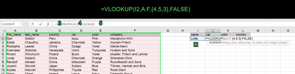
2.2 VLOOKUP Syntax for Multiple Columns

Here’s the enhanced syntax to retrieve data from multiple columns:

=VLOOKUP(lookup_value, table_array, {col1, col2, col3, ...}, [range_lookup])

{col1, col2, col3, …}: An array constant that specifies the column numbers to return. For example, {2, 3, 4} would return values from the second, third, and fourth columns of the table_array.

To enter this as an array formula, after typing the formula, press Ctrl + Shift + Enter (Windows) or Command + Return (Mac). Excel will automatically enclose the formula in curly braces {}.

2.3 Practical Examples

Let’s consider a dataset where you have employee information, including their ID, name, department, and salary. You want to look up an employee by ID and retrieve their name, department, and salary.

Here’s how you can do it:

Data Setup:
- Column A: Employee ID
- Column B: Employee Name
- Column C: Department
- Column D: Salary
Formula:
- If the Employee ID you’re looking up is in cell F2, and your data range is A2:D100, the formula would be:
```
=VLOOKUP(F2, A2:D100, {2, 3, 4}, FALSE)
```
Execution:
- Select three horizontal cells where you want the results to appear.
- Enter the formula in the formula bar.
- Press Ctrl + Shift + Enter (Windows) or Command + Return (Mac).

The name, department, and salary of the employee with the matching ID will populate the selected cells.

3. Comparing Three Columns Using VLOOKUP

Comparing three columns using VLOOKUP requires a slightly more complex approach. The key is to nest VLOOKUP functions or combine them with other logical functions to achieve the desired comparison.

3.1 The Nested VLOOKUP Approach

One effective method is to use nested VLOOKUPs. This involves using the result of one VLOOKUP as the lookup value for another VLOOKUP. The basic logic is:

Compare the first two columns to find matching values.
Compare the matching values from the first comparison with the third column.

3.2 Step-by-Step Guide to Implementing Nested VLOOKUP

Let’s assume you have three columns: A, B, and C, and you want to find values that exist in all three columns.

Data Setup:
- Column A: List 1
- Column B: List 2
- Column C: List 3
Formula:
- In cell D2 (or any empty column), enter the following formula:
```
=IFERROR(VLOOKUP(A2, B:B, 1, FALSE),IFERROR(VLOOKUP(A2, C:C, 1, FALSE),""))
```
- This formula first checks if the value in A2 exists in column B. If it does, it returns the value. If not, it checks if the value in A2 exists in column C. If it does, it returns the value. If neither is true, it returns an empty string.
Drag the Formula:
- Drag the formula down to apply it to all rows in your data.

This will show you the values from column A that are also present in columns B and C. However, this method only confirms if the value from column A exists in B or C. To ensure the value exists in all three columns, you need a slightly different approach.

Here’s a more robust formula:

=IFERROR(VLOOKUP(IFERROR(VLOOKUP(A2,B:B,1,FALSE),""),C:C,1,FALSE),"")

This formula first compares column A to column B, then takes the matching values and compares them to column C. Only values present in all three columns will be returned.

3.3 Handling Errors and Blank Cells

When using nested VLOOKUPs, it’s common to encounter errors like #N/A, which indicates that a lookup value was not found. To handle these errors, use the IFERROR function.

IFERROR: This function allows you to specify a value to return if a formula evaluates to an error.

In the formulas above, IFERROR is used to replace #N/A errors with an empty string (""), making the output cleaner and more readable.

To exclude empty cells, you can use the UNIQUE function (available in Excel 365 or Excel Online) to filter out blank cells before performing the comparison. Alternatively, you can use an advanced array formula:

=IF(ISERROR(SMALL(IF(H2:H66<>"",ROW(H2:H66)-1),ROW(H2:H66)-1)),"", INDEX(H2:H66,MATCH(SMALL(IF(H2:H66<>"",ROW(H2:H66)-1),ROW(H2:H66)-1), IF(H2:H66<>"",ROW(H2:H66)-1),0)))

Replace H2:H66 with your range to apply this formula to your specific dataset. This formula removes blank cells from the comparison, providing a more accurate result.

4. Alternative Methods for Comparing Columns

While VLOOKUP is useful, other functions like MATCH and INDEX can offer more flexibility and efficiency in certain scenarios.

4.1 Using the MATCH Function

The MATCH function returns the position of a lookup value within a range. It can be used to check if a value exists in a column.

Syntax:

=MATCH(lookup_value, lookup_array, [match_type])

lookup_value: The value to search for.
lookup_array: The range to search within.
[match_type]: Specifies how to match the lookup_value. 0 for exact match.

To compare three columns using MATCH, you can combine it with ISNUMBER and IF functions:

=IF(AND(ISNUMBER(MATCH(A2,B:B,0)),ISNUMBER(MATCH(A2,C:C,0))),A2,"")

This formula checks if the value in A2 exists in both columns B and C. If it does, it returns the value; otherwise, it returns an empty string.

4.2 Combining INDEX and MATCH for Flexibility

The INDEX and MATCH functions can be combined to create a more flexible lookup solution compared to VLOOKUP. INDEX returns the value at a given position in a range, while MATCH finds the position of a value.

Syntax:

=INDEX(array, row_num, [column_num])

=MATCH(lookup_value, lookup_array, [match_type])

Combining them:

=INDEX(return_array, MATCH(lookup_value, lookup_array, 0))

This combination allows you to look up values from any column, not just the first one, providing greater flexibility.

4.3 Conditional Formatting for Visual Comparison

Conditional formatting is a powerful feature that allows you to highlight cells based on specific criteria. It’s useful for visually comparing columns and identifying matches or differences.

To compare three columns using conditional formatting:

Select the First Column: Select the range of cells in column A.
Create a New Rule: Go to “Home” > “Conditional Formatting” > “New Rule.”
Use a Formula: Select “Use a formula to determine which cells to format.”
Enter the Formula: Use the following formula:
```
=AND(COUNTIF(B:B,A1)>0,COUNTIF(C:C,A1)>0)
```
Format: Click “Format” and choose a highlighting style (e.g., fill color).
Apply: Click “OK” to apply the rule.

This will highlight the values in column A that also exist in columns B and C, providing a visual comparison.

5. Advanced Techniques and Considerations

For more complex scenarios, advanced techniques such as array formulas and performance optimization are crucial.

5.1 Using Array Formulas for Complex Comparisons

Array formulas can perform calculations on multiple values simultaneously, making them useful for complex comparisons. For example, you can use an array formula to find the intersection of three columns:

{=IFERROR(INDEX(A:A,SMALL(IF(ISNUMBER(MATCH(A:A,B:B,0))*ISNUMBER(MATCH(A:A,C:C,0)),ROW(A:A)),ROW(1:1))),"")}

Remember to enter this formula by pressing Ctrl + Shift + Enter (Windows) or Command + Return (Mac).

5.2 Handling Large Datasets

When working with large datasets, VLOOKUP and other lookup functions can become slow. To improve performance:

Sort Data: Ensure that the lookup column is sorted in ascending order if using approximate match (TRUE).
Use INDEX/MATCH: Consider using INDEX and MATCH instead of VLOOKUP, as they can be faster in some cases.
Optimize Formulas: Avoid using full column references (e.g., A:A) in formulas. Instead, use specific ranges (e.g., A1:A1000).
Disable Automatic Calculation: Turn off automatic calculation while making changes to the spreadsheet, and then re-enable it when finished.

5.3 Performance Optimization Tips

Additional tips to optimize Excel performance:

Use Helper Columns: Create helper columns with pre-calculated values to reduce the complexity of formulas.
Avoid Volatile Functions: Minimize the use of volatile functions like NOW() and TODAY(), which recalculate every time the spreadsheet changes.
Conditional Formatting Wisely: Use conditional formatting sparingly, as it can significantly impact performance, especially with large datasets.

6. Real-World Applications

Comparing three columns in Excel has numerous real-world applications across various industries.

6.1 Inventory Management

In inventory management, you might have three lists: current stock, incoming shipments, and outgoing orders. By comparing these columns, you can identify discrepancies, track stock levels, and ensure timely fulfillment of orders.

Scenario: A company wants to reconcile its inventory data from three sources: the warehouse management system (WMS), the point-of-sale (POS) system, and a manual spreadsheet used by the logistics team.
Columns:
- WMS (Column A): Items recorded in the warehouse management system.
- POS (Column B): Items sold according to the point-of-sale system.
- Logistics (Column C): Items manually tracked by the logistics team.
Objective: Identify which items are consistently recorded across all three systems to ensure data accuracy.
Solution: Use the nested VLOOKUP formula to identify common items:

=IFERROR(VLOOKUP(IFERROR(VLOOKUP(A2,B:B,1,FALSE),""),C:C,1,FALSE),"")

6.2 Financial Analysis

Financial analysts often compare data from different sources to identify trends, discrepancies, and potential risks. Comparing three columns can help reconcile financial statements, track expenses, and monitor key performance indicators.

Scenario: A financial analyst needs to compare monthly revenue data from three different sources: the accounting software, the CRM system, and a manually maintained sales report.
Columns:
- Accounting Software (Column A): Revenue figures from the accounting system.
- CRM System (Column B): Revenue figures from the customer relationship management system.
- Sales Report (Column C): Revenue figures from the sales team’s report.
Objective: Identify discrepancies and ensure that revenue figures are consistent across all three sources.
Solution: Use the MATCH function combined with ISNUMBER and IF functions:

=IF(AND(ISNUMBER(MATCH(A2,B:B,0)),ISNUMBER(MATCH(A2,C:C,0))),A2,"")

6.3 Customer Data Comparison

Businesses often maintain customer data in multiple systems, such as CRM, marketing automation platforms, and customer service databases. Comparing three columns can help identify duplicate records, update missing information, and ensure data consistency across all systems.

Scenario: A marketing team wants to consolidate customer data from three different sources: the CRM system, an email marketing platform, and a customer loyalty program.
Columns:
- CRM (Column A): Customer data from the customer relationship management system.
- Email Platform (Column B): Customer data from the email marketing platform.
- Loyalty Program (Column C): Customer data from the customer loyalty program.
Objective: Identify duplicate customer records and consolidate the data to create a unified customer view.
Solution: Use conditional formatting to highlight common customer records:

Apply the following formula in conditional formatting:

=AND(COUNTIF(B:B,A1)>0,COUNTIF(C:C,A1)>0)

7. Troubleshooting Common Issues

Even with a solid understanding of VLOOKUP, you may encounter common issues. This section addresses how to troubleshoot them effectively.

7.1 #N/A Errors

The #N/A error indicates that VLOOKUP could not find the lookup value in the table array. To resolve this:

Verify Lookup Value: Ensure that the lookup value exists in the first column of the table array.
Check Spelling: Make sure there are no typos or inconsistencies in the lookup value.
Correct Range: Verify that the table array range is correct and includes all relevant data.
Exact Match: If using exact match (FALSE), ensure that the lookup value is an exact match, including case and spaces.
Data Types: Check that the data types of the lookup value and the values in the lookup column are consistent (e.g., both are text or numbers).

7.2 Incorrect Matches

Sometimes, VLOOKUP may return an incorrect match. This typically happens when using approximate match (TRUE) and the lookup column is not sorted correctly.

Sort Data: Ensure that the first column of the table array is sorted in ascending order when using approximate match.
Use Exact Match: If you need an exact match, always use FALSE as the fourth argument in VLOOKUP.
Check Column Index: Verify that the column index number is correct and points to the correct column in the table array.

7.3 Performance Bottlenecks

Performance issues can arise when using VLOOKUP with large datasets. To address these bottlenecks:

Optimize Formulas: Use specific ranges instead of full column references.
Use Helper Columns: Create helper columns with pre-calculated values to reduce formula complexity.
Disable Automatic Calculation: Turn off automatic calculation while making changes to the spreadsheet.
Consider Alternatives: Use INDEX and MATCH as they can be faster than VLOOKUP in some cases.
Excel Settings: Adjust Excel settings to allocate more memory and processing power to the spreadsheet.

8. Automating Data Import to Excel

To streamline the data comparison process, automate the data import to Excel using tools like Power Query or third-party connectors.

8.1 Using Power Query

Power Query is a powerful data transformation and integration tool built into Excel. It allows you to import data from various sources, clean and transform it, and load it into Excel for analysis.

To use Power Query:

Get Data: Go to “Data” > “Get & Transform Data” > “Get Data.”
Choose Data Source: Select the data source (e.g., CSV file, database, web page).
Transform Data: Use the Power Query Editor to clean and transform the data as needed.
Load Data: Load the data into an Excel worksheet.

8.2 Third-Party Tools for Data Integration

Several third-party tools can automate data import to Excel, such as:

Coupler.io: Automate data imports from various sources with refresh schedules.
Zapier: Connect Excel with other apps to automate data transfer.
Microsoft Power Automate: Create automated workflows to import and transform data.

Using these tools can save time and effort, ensuring that your data is always up-to-date and ready for comparison.

9. Excel Online vs. Desktop Version

When comparing data in Excel, it’s essential to consider whether you’re using the online or desktop version, as there are some differences in functionality and collaboration benefits.

9.1 Differences in Functionality

Array Formulas: In Excel Online, array formulas often work more seamlessly without needing to press Ctrl + Shift + Enter. The formula automatically spills into the adjacent cells.
Add-ins: Some add-ins available in the desktop version may not be available or fully functional in Excel Online.
Performance: The desktop version generally offers better performance with large datasets due to its ability to leverage local processing power.
Advanced Features: Certain advanced features, such as Power Query and VBA macros, may have limited functionality in Excel Online.

9.2 Cloud Collaboration Benefits

Excel Online offers several collaboration benefits:

Real-Time Collaboration: Multiple users can work on the same spreadsheet simultaneously.
Accessibility: Access your spreadsheets from anywhere with an internet connection.
Version History: Track changes and revert to previous versions.
Sharing: Easily share spreadsheets with others and control access permissions.

10. Frequently Asked Questions (FAQ)

Q1: Can VLOOKUP compare values across multiple worksheets?
Yes, VLOOKUP can compare values across multiple worksheets by referencing the appropriate worksheet in the table_array argument.

Q2: How do I handle case-sensitive lookups with VLOOKUP?
VLOOKUP is not case-sensitive by default. To perform case-sensitive lookups, use the FIND function in combination with INDEX and MATCH.

Q3: Is there a limit to the number of columns VLOOKUP can compare?
VLOOKUP itself does not compare columns but retrieves data from a specified column. Comparing multiple columns often involves nesting or combining VLOOKUP with other functions, which can become complex but does not have a hard limit.

Q4: How can I improve VLOOKUP performance with large datasets?
To improve performance, use specific ranges, sort data, consider using INDEX and MATCH, and disable automatic calculations while making changes.

Q5: Can I use VLOOKUP to compare dates?
Yes, VLOOKUP can compare dates as long as the date formats are consistent.

Q6: What is the difference between VLOOKUP and HLOOKUP?
VLOOKUP looks up values vertically in the first column of a range, while HLOOKUP looks up values horizontally in the first row of a range.

Q7: How do I handle errors when using VLOOKUP?
Use the IFERROR function to replace errors with a more meaningful value or an empty string.

Q8: Can I use wildcards with VLOOKUP?
Yes, you can use wildcards like * (asterisk) and ? (question mark) in the lookup_value argument to perform partial matches.

Q9: How do I lookup the last value in a column using VLOOKUP?
You cannot directly lookup the last value with VLOOKUP. However, you can combine it with other functions like INDEX, MATCH, and COUNTA to achieve this.

Q10: Is VLOOKUP available in all versions of Excel?
VLOOKUP is available in all versions of Excel, including Excel Online and desktop versions.

11. Conclusion

Comparing three columns in Excel using VLOOKUP and alternative methods can significantly enhance your data analysis capabilities. Whether you’re reconciling financial statements, managing inventory, or consolidating customer data, mastering these techniques will enable you to make more informed decisions. Remember to optimize your formulas, handle errors effectively, and consider automating data import to streamline your workflow.

For more in-depth comparisons and decision-making tools, visit COMPARE.EDU.VN at 333 Comparison Plaza, Choice City, CA 90210, United States, or contact us via WhatsApp at +1 (626) 555-9090. Our website provides comprehensive comparisons to help you make the best choices. Don’t struggle with data; let compare.edu.vn simplify your decision-making process.