Discover the precise formula to use in Excel for comparing two columns effectively with this guide from COMPARE.EDU.VN, ensuring accuracy and saving time. This comprehensive tutorial offers practical solutions, enhancing data analysis and comparison tasks with efficient methods and powerful tools, ultimately providing a seamless experience. Explore the advantages of leveraging spreadsheet analysis and data comparison techniques.
1. Understanding the Need for Column Comparison in Excel
Excel is more than just a spreadsheet program; it’s a powerful tool for data management, analysis, and decision-making. Comparing two columns within Excel is crucial for various tasks, ranging from identifying duplicates to verifying data integrity. Whether you are managing inventories, analyzing sales figures, or maintaining customer databases, knowing What Formula To Use In Excel To Compare Two Columns can significantly improve your workflow. Manually sifting through rows of data is not only time-consuming but also prone to error. Excel provides several formulas and features that automate this process, ensuring accuracy and efficiency. This is where COMPARE.EDU.VN can help you find the best methods and formulas for your specific needs.
2. Basic Comparison Using the Equals Operator
One of the simplest methods to compare two columns in Excel is by using the equals operator (=). This method performs a row-by-row comparison, returning TRUE if the values in the two columns match and FALSE if they don’t. Here’s how to implement it:
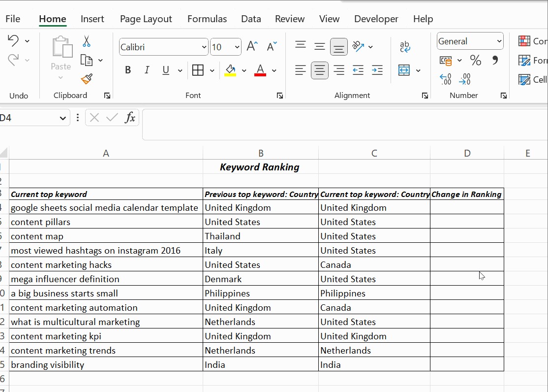
- Open your Excel sheet: Make sure you have the two columns you want to compare side by side.
- Select a cell in a new column where you want the results to appear.
- Enter the formula: In the selected cell, type
=A1=B1(assuming your data starts in row 1 and the columns you are comparing are A and B). - Press Enter: The cell will display either TRUE or FALSE.
- Drag the formula: Click and drag the bottom-right corner of the cell down to apply the formula to the rest of the rows.
This method is straightforward and useful for a quick overview of matching and non-matching data. However, it is case-insensitive, meaning it will treat “Apple” and “apple” as the same.
3. Enhanced Comparison with the IF Function
The IF function in Excel allows you to create more descriptive results than just TRUE or FALSE. By using the IF function, you can return custom messages like “Match” or “No Match,” making the results easier to interpret. The syntax is as follows:
=IF(logical_test, value_if_true, value_if_false)
Here’s how to use it for comparing two columns:
- Select a cell in a new column.
- Enter the formula: Type
=IF(A1=B1, "Match", "No Match"). - Press Enter: The cell will display “Match” if the values in columns A and B are the same, and “No Match” if they are different.
- Drag the formula down to apply it to all rows.
This method offers more clarity, especially when dealing with large datasets. You can customize the messages to fit your specific needs, such as “Duplicate” or “Unique,” depending on what you are looking for.
4. Case-Sensitive Comparison Using the EXACT Function
In many scenarios, the case of the text matters. For instance, when comparing usernames, product codes, or other identifiers, “ID123” is different from “id123.” The EXACT function in Excel provides a case-sensitive comparison. The syntax is:
=EXACT(text1, text2)
The EXACT function returns TRUE if the two text strings are exactly the same, including the case, and FALSE otherwise. To use it in combination with the IF function:
- Select a cell in a new column.
- Enter the formula: Type
=IF(EXACT(A1, B1), "Match", "No Match"). - Press Enter.
- Drag the formula down to apply it to all rows.
This ensures that only the exact matches, including the case, are flagged as “Match,” providing a more accurate comparison when case sensitivity is important.
5. Highlighting Differences with Conditional Formatting
Conditional formatting is a powerful feature in Excel that allows you to automatically format cells based on certain criteria. This can be incredibly useful for visually identifying differences between two columns. Here’s how to use conditional formatting to highlight unique or duplicate values:
- Select the two columns you want to compare.
- Go to Home > Conditional Formatting > Highlight Cells Rules.
- Choose Duplicate Values or Unique Values depending on what you want to highlight.
- Duplicate Values: Highlights cells that appear in both columns.
- Unique Values: Highlights cells that are unique to each column.
- Choose a formatting style: Select the color and style you want to use for highlighting.
This method provides a visual way to quickly identify matching or differing data without adding extra columns or formulas.
5.1. Custom Conditional Formatting
For more complex scenarios, you can use custom conditional formatting rules. For instance, to highlight rows where the values in two columns do not match:
- Select the range of cells you want to format (e.g., both columns A and B).
- Go to Home > Conditional Formatting > New Rule.
- Select “Use a formula to determine which cells to format.”
- Enter the formula: Type
=A1<>B1(assuming your data starts in row 1). - Click Format to choose the formatting style (e.g., fill color, font color).
- Click OK to apply the rule.
This will highlight all the rows where the values in column A do not match the values in column B, making it easy to spot discrepancies.
6. Using Lookup Functions for Advanced Comparisons
Lookup functions like VLOOKUP, HLOOKUP, and XLOOKUP are invaluable for comparing columns based on specific criteria. These functions search for a value in one column and return a corresponding value from another column.
6.1. VLOOKUP for Column Comparison
VLOOKUP (Vertical Lookup) is used to find a value in the first column of a range and return a value from a specified column in the same row. The syntax is:
=VLOOKUP(lookup_value, table_array, col_index_num, [range_lookup])
- lookup_value: The value you want to find.
- table_array: The range of cells in which to search.
- col_index_num: The column number in the range from which to return a value.
- range_lookup: Optional. TRUE for approximate match, FALSE for exact match.
For example, to check if the values in column A exist in column B and return a corresponding value from column B:
- Select a cell in a new column.
- Enter the formula:
=VLOOKUP(A1, B:B, 1, FALSE). - Press Enter.
- Drag the formula down to apply it to all rows.
If VLOOKUP finds a match, it returns the matching value from column B. If it doesn’t find a match, it returns #N/A. You can use the ISNA function to handle the #N/A errors and display a custom message:
=IF(ISNA(VLOOKUP(A1, B:B, 1, FALSE)), "Not Found", "Found")
6.2. XLOOKUP for Modern Excel Versions
XLOOKUP is a more versatile and modern version of VLOOKUP and HLOOKUP. It simplifies the lookup process and offers better flexibility. The syntax is:
=XLOOKUP(lookup_value, lookup_array, return_array, [if_not_found], [match_mode], [search_mode])
- lookup_value: The value to search for.
- lookup_array: The range to search within.
- return_array: The range from which to return a value.
- if_not_found: Optional. The value to return if no match is found.
- match_mode: Optional. Specifies the type of match (0 for exact match).
- search_mode: Optional. Specifies the search direction.
Using XLOOKUP to compare two columns:
- Select a cell in a new column.
- Enter the formula:
=XLOOKUP(A1, B:B, B:B, "Not Found"). - Press Enter.
- Drag the formula down to apply it to all rows.
XLOOKUP will return the matching value from column B if found, and “Not Found” if not found, making the comparison straightforward and easy to understand.
7. COUNTIF and COUNTIFS for Counting Matches
Sometimes, you might want to count how many times a value from one column appears in another column. The COUNTIF and COUNTIFS functions are perfect for this.
7.1. Using COUNTIF
COUNTIF counts the number of cells within a range that meet a given criterion. The syntax is:
=COUNTIF(range, criteria)
To count how many times the values in column A appear in column B:
- Select a cell in a new column.
- Enter the formula:
=COUNTIF(B:B, A1). - Press Enter.
- Drag the formula down to apply it to all rows.
The result will show how many times each value in column A appears in column B. If the count is 0, it means the value does not exist in column B.
7.2. Using COUNTIFS
COUNTIFS is used to count cells based on multiple criteria. This is useful when you need to compare columns based on more than one condition. The syntax is:
=COUNTIFS(criteria_range1, criteria1, [criteria_range2, criteria2], ...)
For example, if you want to count how many times values in column A match values in column B and column C:
- Select a cell in a new column.
- Enter the formula:
=COUNTIFS(B:B, A1, C:C, A1). - Press Enter.
- Drag the formula down to apply it to all rows.
This will return the count of instances where the values in column A match both column B and column C in the same row.
8. Array Formulas for Complex Comparisons
Array formulas can perform complex calculations on multiple values at once. They are particularly useful for comparing entire columns without dragging formulas down.
8.1. Comparing Two Columns for Differences Using Array Formulas
To identify the differences between two columns using an array formula:
- Select a range of cells where you want the results to appear. The range should be the same size as the columns you are comparing.
- Enter the formula:
={IF(A1:A10=B1:B10, "Match", "No Match")}. - Press Ctrl + Shift + Enter to enter the formula as an array formula. Excel will automatically add curly braces
{}around the formula.
This will compare each row in columns A and B and display “Match” or “No Match” in the selected range.
8.2. Finding Unique Values Using Array Formulas
To find unique values in column A that do not exist in column B:
- Select a range of cells where you want the results to appear.
- Enter the formula:
={IF(ISERROR(MATCH(A1:A10, B1:B10, 0)), A1:A10, "")}. - Press Ctrl + Shift + Enter to enter the formula as an array formula.
This formula uses the MATCH function to find if each value in column A exists in column B. If MATCH returns an error (meaning the value is not found), the formula returns the value from column A; otherwise, it returns an empty string.
9. Power Query for Advanced Data Comparison
Power Query is a powerful data transformation and analysis tool in Excel. It allows you to import data from various sources, clean and transform it, and perform complex comparisons.
9.1. Comparing Columns Using Power Query
- Load your data into Power Query:
- Select your data range.
- Go to Data > From Table/Range.
- Load the second column or table into Power Query.
- Merge the queries:
- Go to Home > Merge Queries.
- Select the two tables you want to merge.
- Choose the columns to compare (e.g., column A from the first table and column B from the second table).
- Select the Join Kind. For example, choose “Left Outer” to keep all rows from the first table and matching rows from the second table.
- Expand the merged column:
- Click the Expand icon in the header of the merged column.
- Select the columns you want to include in the final result.
- Compare the columns:
- Add a custom column to compare the values.
- Go to Add Column > Custom Column.
- Enter a formula like
if [ColumnA] = [ColumnB] then "Match" else "No Match".
- Load the result back into Excel:
- Go to Home > Close & Load > Close & Load To.
- Select where you want to load the data.
Power Query provides a robust and flexible way to compare columns, especially when dealing with large datasets or complex data transformations.
10. Real-World Examples and Use Cases
To illustrate the practical application of these formulas, let’s consider a few real-world examples:
10.1. Inventory Management
Imagine you have two lists of inventory items: one from your warehouse and one from your sales records. You want to identify discrepancies between the two lists. By using the techniques described above, you can quickly identify missing items, overstocked items, and data entry errors.
- Use VLOOKUP or XLOOKUP to check if each item in the sales record exists in the warehouse list.
- Use COUNTIF to count how many times each item appears in both lists.
- Use conditional formatting to highlight items that are only present in one list.
10.2. Customer Database Management
You have two customer databases and want to merge them, ensuring there are no duplicate entries.
- Use EXACT to compare customer names, ensuring case sensitivity.
- Use COUNTIF to identify duplicate entries.
- Use conditional formatting to highlight potential duplicates for manual review.
10.3. Financial Data Analysis
You need to compare two columns of financial data, such as monthly expenses versus budget.
- Use the equals operator and IF to quickly identify matching and non-matching amounts.
- Use conditional formatting to highlight variances that exceed a certain threshold.
- Use array formulas to calculate the total variance between the two columns.
11. Optimizing Performance for Large Datasets
When working with large datasets in Excel, performance can become an issue. Here are some tips to optimize performance when comparing columns:
- Use efficient formulas: VLOOKUP and XLOOKUP can be slow on large datasets. Consider using INDEX and MATCH as an alternative.
- Avoid volatile functions: Functions like NOW() and RAND() recalculate every time the spreadsheet changes, which can slow down performance.
- Use helper columns: Break down complex formulas into smaller, more manageable steps using helper columns.
- Turn off automatic calculations: Manually calculate the spreadsheet when you are ready by pressing F9.
- Use Power Query: Power Query is designed to handle large datasets efficiently and can significantly improve performance.
12. Common Mistakes to Avoid
When comparing columns in Excel, there are several common mistakes to avoid:
- Ignoring case sensitivity: Use the EXACT function when case matters.
- Not locking ranges in lookup functions: Use absolute references ($) to lock the ranges in VLOOKUP and XLOOKUP.
- Not handling errors: Use ISNA or IFERROR to handle errors like #N/A.
- Using inefficient formulas on large datasets: Consider using Power Query or more efficient formulas like INDEX and MATCH.
- Overlooking data types: Ensure that the data types in the columns you are comparing are consistent (e.g., numbers, text, dates).
13. Conclusion: Choosing the Right Formula for Your Needs
In conclusion, knowing what formula to use in Excel to compare two columns is essential for data analysis and management. Whether you’re using the basic equals operator, the versatile IF function, or the advanced lookup functions like VLOOKUP and XLOOKUP, Excel offers a range of tools to suit your specific needs. By understanding these methods and avoiding common mistakes, you can ensure accurate and efficient column comparisons, saving time and improving the quality of your data analysis. Remember to visit COMPARE.EDU.VN for more in-depth guides and comparisons of different Excel techniques.
14. COMPARE.EDU.VN: Your Partner in Data-Driven Decisions
At COMPARE.EDU.VN, we understand the importance of making informed decisions based on accurate data. That’s why we provide comprehensive comparisons and guides to help you master tools like Excel and make the most of your data. Whether you’re comparing products, services, or data sets, our goal is to empower you with the knowledge and resources you need to succeed. Contact us at 333 Comparison Plaza, Choice City, CA 90210, United States or via Whatsapp at +1 (626) 555-9090.
Ready to take your data analysis skills to the next level? Visit COMPARE.EDU.VN today to explore more resources and comparisons.
Frequently Asked Questions
1. How do I compare two columns in Excel to see if they match?
You can use the formula =A1=B1 to compare two cells in columns A and B. Drag the formula down to compare the entire columns. The result will be TRUE if they match and FALSE if they don’t. Alternatively, use =IF(A1=B1, "Match", "No Match") for a more descriptive result.
2. How can I perform a case-sensitive comparison in Excel?
Use the EXACT function for a case-sensitive comparison. The formula =IF(EXACT(A1, B1), "Match", "No Match") will return “Match” only if the text in cells A1 and B1 are exactly the same, including the case.
3. How do I highlight differences between two columns in Excel?
Use conditional formatting to highlight differences. Select the columns, go to Home > Conditional Formatting > New Rule, and use the formula =A1<>B1 to highlight rows where the values don’t match.
4. What is the best way to compare two columns for differences in large datasets?
For large datasets, consider using Power Query. Load the data into Power Query, merge the columns, and add a custom column to compare the values. Power Query is designed to handle large datasets efficiently.
5. How can I count the number of matches between two columns in Excel?
Use the COUNTIF function to count the number of times a value from one column appears in another column. For example, =COUNTIF(B:B, A1) will count how many times the value in cell A1 appears in column B.
6. Can I use VLOOKUP to compare two columns?
Yes, you can use VLOOKUP to check if values in one column exist in another. The formula =VLOOKUP(A1, B:B, 1, FALSE) will search for the value in cell A1 within column B and return the matching value if found. If not found, it returns #N/A, which you can handle with IFERROR.
7. What is the XLOOKUP function and how is it better than VLOOKUP?
XLOOKUP is a modern lookup function that is more versatile and easier to use than VLOOKUP. It simplifies the lookup process and offers better flexibility. For example, =XLOOKUP(A1, B:B, B:B, "Not Found") will search for the value in cell A1 within column B and return the matching value if found, or “Not Found” if not found.
8. How do I find unique values in one column that do not exist in another column?
Use an array formula to find unique values. Select a range of cells and enter the formula ={IF(ISERROR(MATCH(A1:A10, B1:B10, 0)), A1:A10, "")}. Press Ctrl + Shift + Enter to enter the formula as an array formula.
9. What are some common mistakes to avoid when comparing columns in Excel?
Common mistakes include ignoring case sensitivity, not locking ranges in lookup functions, not handling errors, using inefficient formulas on large datasets, and overlooking data types.
10. Where can I find more resources and comparisons of Excel techniques?
Visit compare.edu.vn for in-depth guides and comparisons of different Excel techniques. We offer comprehensive resources to help you master Excel and make the most of your data.