Comparing if two columns match in Excel is a common task for data analysis, and COMPARE.EDU.VN is here to guide you. This guide offers effective methods to streamline your data analysis, revealing hidden patterns and ensuring data integrity. Discover the best approaches for comparing columns and maximizing Excel’s capabilities for informed decision-making with effective formulas and formatting techniques.

At COMPARE.EDU.VN, we understand the importance of accurate data comparison. Comparing data sets, contrasting information, and contrasting values are critical for any professional working with data.

1. Understanding the Need for Column Comparison in Excel

Excel is an indispensable tool for data storage, manipulation, and informed decision-making. Its versatility allows users to efficiently manage and analyze large datasets. Data analysts rely on Excel to gather crucial information that drives strategic marketing and sales decisions.

• Data Integrity: Ensuring data accuracy across spreadsheets.
• Identifying Discrepancies: Pinpointing missing or inconsistent information.
• Streamlining Analysis: Automating comparisons to save time and reduce errors.
• Supporting Decisions: Providing reliable data for informed choices.

When cells lack information, it can significantly impact the integrity of analyses and outcomes. Spreadsheets often contain vast amounts of data, and multiple spreadsheets are interconnected, making manual comparisons impractical. A data analyst must frequently compare columns within the same or different spreadsheets. Manually comparing columns is a time-consuming task that can take hours or even days to uncover missing data. Therefore, comparing two columns in Excel is essential for determining whether a cell contains data. Excel can display results as TRUE/FALSE, Match/Not Match, or custom messages defined by the user, enhancing clarity and efficiency.

2. Essential Methods to Compare Two Columns in Excel

Comparing data in two columns, tables, or spreadsheets is often necessary to identify missing or duplicate data. The method chosen depends on the desired outcome. Effective comparison techniques include:

• Highlighting unique or duplicate values using built-in functions.
• Displaying unique or duplicate values using conditional formatting or formulas.
• Performing row-by-row comparisons.
• Utilizing LOOKUP formulas.

These methods provide a comprehensive toolkit for efficiently comparing data and extracting valuable insights.

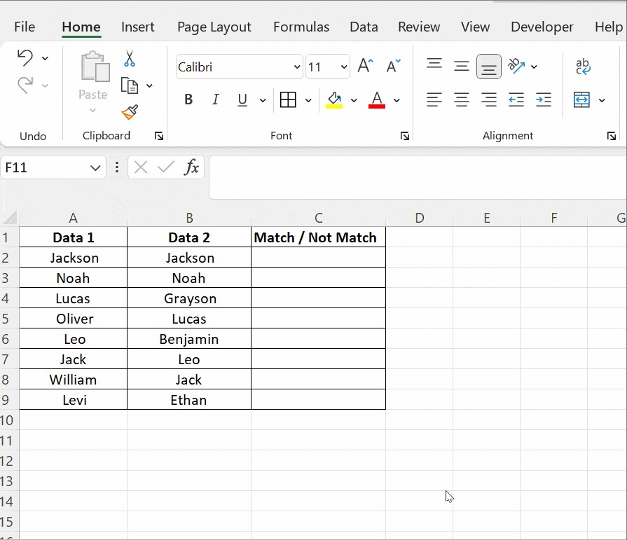
3. Comparing Two Columns with the Equals Operator

The equals operator (=) allows row-by-row comparisons, indicating matching data with a “Match” or “Not Match” result. For example, the formula =A2=B2 compares the values in cells A2 and B2, returning TRUE if they match and FALSE if they differ.

3.1 Step-by-Step Guide

1. Enter the Formula: In cell C2, enter the formula =A2=B2 and press Enter.
2. Apply to All Rows: Drag the formula down to the end of the table.
3. Analyze Results: The formula returns TRUE for matching values and FALSE for different values.

This method provides a quick and straightforward way to identify matching entries across two columns.

4. Using the IF Condition for Column Comparison

The IF condition in Excel provides a versatile approach to comparing two columns. The basic formula, =IF(A2=B2,”Match”,””), checks if the values in cells A2 and B2 match. If they do, the formula returns “Match”; otherwise, it leaves the cell blank.

4.1 Identifying Mismatching Values

To identify mismatching values, modify the formula to =IF(A2=B2,”Match”,”Not a Match”). This version returns “Match” for matching values and “Not a Match” for differing values.

4.2 Comparing for Differences

To specifically check for differences, replace the equals sign with the non-equality sign (<>). The formula becomes =IF(A2<>B2,”Match”,”Not a Match”). This setup returns “Match” when values differ and “Not a Match” when they are identical.

5. Utilizing the EXACT() Function for Case-Sensitive Comparisons

The EXACT() function is crucial when comparing two columns in Excel and case sensitivity is essential. This function distinguishes between uppercase and lowercase letters, ensuring precise comparisons.

5.1 Understanding the EXACT() Function

The EXACT() function compares two text strings and returns TRUE if they are identical, including case, and FALSE otherwise. Formatting differences are ignored. The syntax is =EXACT(text1, text2), where both arguments are required.

5.2 Practical Example

Consider two columns, Data1 and Data2, both containing the text “Nova Scotia,” but potentially with different capitalization.

	Column A (Data1)	Column B (Data2)
Row 2	Nova Scotia	Nova Scotia

5.3 Case-Insensitive Comparison

The formula =IF(A2=B2, “Match”, “Mismatch”) in cell C2 returns “Match” because it is case-insensitive.

5.4 Case-Sensitive Comparison

To perform a case-sensitive comparison, use the formula =IF(EXACT(A2, B2), “Match”, “Mismatch”).

5.5 How It Works

1. Inner Function Execution: The EXACT() function executes first, comparing the text strings.
2. Result Returned: The EXACT() function returns TRUE or FALSE to the outer IF function.
3. IF Condition Evaluation: If EXACT() returns TRUE, the IF condition returns “Match”; otherwise, it returns “Mismatch.”

The EXACT() function is essential for scenarios requiring precise, case-sensitive comparisons, ensuring accurate data analysis.

6. Comparing Columns with Conditional Formatting

Conditional formatting is an effective way to visually highlight matching or unique values in two columns.

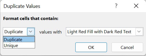
6.1 Step-by-Step Guide

1. Select Data: Select the entire table.
2. Access Conditional Formatting: Go to Home → Styles → Conditional Formatting → Highlight Cell Rules → Duplicate Values.
3. Choose Formatting Condition: In the dialog box, choose Duplicate or Unique from the drop-down menu.

4. Select Format: Choose a formatting option such as filling with color, changing the text color, or altering the cell border.
5. Custom Format: For custom colors, select Custom Format.

6.2 Highlighting Duplicate Values

To highlight values present in both columns, select Duplicate and apply the desired formatting.

6.3 Highlighting Unique Values

To highlight unique values, select Unique from the drop-down list and apply the formatting.

6.4 Clearing Formatting

To remove conditional formatting, click Conditional Formatting → Clear Rules → Clear Rules from Selected Cells.

Conditional formatting is useful for smaller tables where a third column is not needed, providing a visual representation of matching or unique data.

7. Leveraging Lookup Functions to Compare Two Columns

Lookup functions like VLOOKUP, HLOOKUP, and XLOOKUP search for a value in a row or column and return a corresponding value from another row or column. VLOOKUP is particularly useful for comparing two columns.

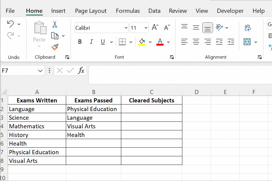
7.1 Example Using VLOOKUP()

Consider a scenario where Column A lists exams taken by a student, and Column B lists subjects the student passed. The goal is to determine which subjects the student cleared.

7.2 Applying VLOOKUP()

1. Enter the Formula: In cell C2, enter the formula =VLOOKUP(A2, $B$2:$B$5, 1, 0).
2. Apply to All Rows: Drag the formula down to apply it to all cells in Column C.

7.3 Understanding the Formula

• VLOOKUP(A2,…): Takes the value in cell A2 (the exam subject).
• VLOOKUP(A2, $B$2:$B$5,…): Compares the value with all values in cells B2 to B5 (the list of passed subjects). The absolute reference ($) locks the cell range.
• VLOOKUP(A2, $B$2:$B$5, 1,…): The col_index_num argument specifies the column to compare from the lookup value. In this case, it is 1, as the passed subjects list is in the adjacent column.
• VLOOKUP(A2, $B$2:$B$5, 1, 0): The last argument specifies whether to find an exact match (0) or the closest match in ascending order (1). Here, 0 ensures an exact match.

7.4 Interpreting Results

Column C will show the cleared subjects. Cells where the subject was not cleared will display #N/A, indicating that the subject was not found in the list of passed subjects.

8. More Methods to Compare Two Columns

8.1 Using “Go To Special”

The “Go To Special” feature in Excel allows you to quickly identify differences between two columns.

1. Select Columns: Select both columns of data.
2. Go To Special: Select Home → Find & Select → Go To Special → Row Differences and click OK.

The matching cells will appear white, while unmatched cells will be gray, providing a clear visual comparison.

8.2 Combining IF with AND/OR Conditions

To find matches across multiple columns, use IF with AND/OR statements.

8.2.1 Finding Full Matches

To find rows where all cells have the same values across multiple columns, use the formula =IF(AND(A2=B2, A2=C2), “Full match”, “”).

8.2.2 Finding Any Matches

To find rows where at least two cells match, use the formula =IF(OR(A2=B2, B2=C2, A2=C2), “Match”, “”).

8.3 Using INDEX-MATCH Function

The INDEX-MATCH function can compare two columns in different tables and pull matching entries from the comparing table. This function is more flexible than VLOOKUP.

8.3.1 Syntax and Usage

The formula =INDEX(ColumnB, MATCH(D2, ColumnA, 0)) compares values in column D with those in column A. If a match is found, it pulls the corresponding value from column B.

8.3.2 How It Works

The MATCH() function searches for values from column D in column A. If a match is found, it returns the position of the match. The INDEX() function then uses this position to retrieve the corresponding value from column B. If no match is found, it returns #N/A.

9. Practical Applications of Column Comparison in Excel

Comparing columns in Excel is useful in a variety of real-world scenarios:

• Data Validation: Ensuring data consistency between different sources.
• Inventory Management: Comparing stock levels across different warehouses.
• Financial Analysis: Identifying discrepancies in financial records.
• Customer Relationship Management: Comparing customer data across different databases.
• Research Analysis: Validating data collected from different experiments or surveys.
• HR Management: Comparing employee data across different departments.

10. Best Practices for Column Comparison in Excel

To ensure accurate and efficient column comparisons, follow these best practices:

• Prepare Your Data: Ensure data is clean and consistently formatted before comparison.
• Choose the Right Method: Select the comparison method based on the specific requirements of your task.
• Use Absolute References: When using formulas like VLOOKUP, use absolute references to lock cell ranges.
• Test Your Formulas: Always test your formulas on a small subset of data before applying them to the entire dataset.
• Document Your Steps: Keep a record of the steps you take and the formulas you use for future reference.
• Handle Errors: Be prepared to handle errors such as #N/A and understand what they mean in the context of your comparison.
• Automate Where Possible: Use macros or VBA to automate repetitive comparison tasks.

11. Why Choose COMPARE.EDU.VN for Your Data Analysis Needs?

At COMPARE.EDU.VN, we understand the critical role of accurate data analysis in driving informed decision-making. Whether you’re a student, a professional, or an entrepreneur, our platform provides the resources and tools you need to master data comparison in Excel.

• Comprehensive Guides: Our in-depth articles cover a wide range of data analysis techniques, including column comparison methods.
• Practical Examples: We provide real-world examples and step-by-step tutorials to help you apply these techniques in your own projects.
• Expert Insights: Our team of data analysis experts shares their knowledge and experience to help you overcome challenges and achieve your goals.
• Time-Saving Resources: We offer templates, checklists, and other resources to help you streamline your data analysis workflow and save time.
• Continuous Learning: Our platform is constantly updated with new content and resources to help you stay ahead of the curve.

12. Frequently Asked Questions

1. How do I compare two columns in Excel to find differences?

To compare two columns and find differences, select both columns, go to Home → Find & Select → Go To Special → Row Differences, and click OK. The unmatched cells will be highlighted.

2. How can I compare two columns in Excel using the IF condition?

Use the formula =IF(A2=B2, “Match”, “Mismatch”) to compare values in cells A2 and B2. Modify the formula to =IF(A2<>B2, “Match”, “Mismatch”) to find differences.

3. Can I compare two columns in Excel using the Index-Match function?

Yes, use the formula =INDEX(ColumnB, MATCH(D2, ColumnA, 0)) to compare values in column D with those in column A. If a match is found, it pulls the corresponding value from column B.

4. How do I perform a case-sensitive comparison in Excel?

Use the EXACT() function. The formula =IF(EXACT(A2, B2), “Match”, “Mismatch”) compares values in cells A2 and B2, considering case sensitivity.

5. How can I highlight duplicate values in two columns?

Select the data, go to Home → Styles → Conditional Formatting → Highlight Cell Rules → Duplicate Values, and choose the desired formatting.

6. What is the purpose of absolute references in VLOOKUP?

Absolute references ($) lock cell ranges, ensuring the correct range is used when the formula is dragged down or across. For example, $B$2:$B$5 ensures the range B2:B5 remains constant.

7. How do I handle #N/A errors in VLOOKUP?

N/A errors indicate that the lookup value was not found. Use the IFERROR() function to handle these errors, such as =IFERROR(VLOOKUP(A2, $B$2:$B$5, 1, 0), “Not Found”).

8. Can I use conditional formatting to highlight unique values in two columns?

Yes, select the data, go to Home → Styles → Conditional Formatting → Highlight Cell Rules → Unique Values, and choose the desired formatting.

9. What are some practical applications of column comparison in Excel?

Practical applications include data validation, inventory management, financial analysis, customer relationship management, research analysis, and HR management.

10. What if the two columns I am comparing are in different Excel sheets?

When comparing two columns from different sheets, you need to specify the sheet name in the formula. For example, to compare column A in “Sheet1” with column A in “Sheet2”, you can use the following formula in “Sheet1”: =IF(A1=Sheet2!A1, "Match", "No Match"). You can drag this formula down to compare all corresponding rows. For conditional formatting, select the range in one sheet, then create a new rule using a formula, referring to the corresponding cells in the other sheet. This approach ensures that the comparison is accurately made across different sheets within the same Excel workbook.

Conclusion

Comparing two columns in Excel is an essential skill for anyone working with data. Whether you’re ensuring data integrity, identifying discrepancies, or streamlining analysis, mastering these techniques will enable you to make informed decisions and gain deeper insights from your data. At COMPARE.EDU.VN, we are committed to providing you with the resources and knowledge you need to excel in data analysis.

For further assistance and to explore more data comparison methods, reach out to us. Visit compare.edu.vn or contact us at 333 Comparison Plaza, Choice City, CA 90210, United States, or via WhatsApp at +1 (626) 555-9090. Our team is here to help you navigate the intricacies of Excel and data analysis, ensuring you can effectively compare and contrast information and make data-driven decisions.