Comparing columns in Excel for matches is a crucial task for data analysis, cleaning, and reporting. COMPARE.EDU.VN provides a comprehensive overview of different methods to achieve this efficiently, ensuring accuracy and saving valuable time. Discover various Excel functionalities to compare data, identify matches, and highlight discrepancies within your spreadsheets to make better data driven decision.
1. Understanding the Basics of Comparing Columns in Excel
Comparing columns in Excel involves examining data sets side-by-side to identify similarities, differences, and patterns. This process is essential for ensuring data integrity, merging information, and extracting valuable insights. Whether you’re comparing product lists, customer databases, or financial records, mastering the art of column comparison in Excel is invaluable. This operation involves numerous excel features to identify the differences like conditional formatting, using equal operators and other excel formulas to compare and analyze the data.
1.1 Why is Comparing Columns Important?
Comparing columns allows users to:
- Identify duplicate entries.
- Verify data consistency.
- Merge information from multiple sources.
- Analyze trends and patterns.
- Detect errors and inconsistencies.
1.2 Basic Concepts
Before diving into specific methods, it’s important to understand some basic Excel concepts:
- Cell Referencing: Understanding how to refer to cells and ranges (e.g., A1, B2:B10).
- Formulas: Knowing how to write and use formulas for calculations and comparisons.
- Functions: Familiarizing yourself with built-in functions like
IF,VLOOKUP, andCOUNTIF. - Conditional Formatting: Using rules to highlight cells based on their values.
2. Methods for Comparing Two Columns in Excel
There are several methods to compare two columns in Excel, each with its own advantages and use cases. Here, COMPARE.EDU.VN, explores five effective techniques.
2.1 Conditional Formatting
Conditional formatting is a simple yet powerful way to highlight matches and differences in your data.
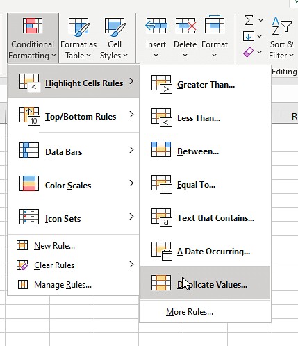
2.1.1 Steps to Use Conditional Formatting
- Select the Columns: Highlight the columns you want to compare.
- Navigate to Conditional Formatting: Go to the “Home” tab, click “Conditional Formatting,” and choose “Highlight Cells Rules.”
-
Select Duplicate or Unique Values:
- To find matching values, select “Duplicate Values.”
- To find unique values, select “Unique Values.”
-
Choose Formatting Style: Select a formatting style (e.g., fill color, font color) to highlight the values.
-
Apply and View Results: Click “OK” to apply the formatting.
2.1.2 Example
Suppose you have two columns, A and B, with customer IDs. To highlight duplicate IDs, select both columns, navigate to “Conditional Formatting,” choose “Highlight Cells Rules,” select “Duplicate Values,” and choose a fill color. All matching IDs will be highlighted.
2.1.3 Advantages and Disadvantages
- Advantages:
- Simple and quick to implement.
- Visually highlights matches and differences.
- Disadvantages:
- Doesn’t provide a summary or count of matches.
- Limited customization options.
2.2 Using the Equals Operator
The equals operator (=) is a straightforward way to compare individual cells and return a TRUE or FALSE result.
2.2.1 Steps to Use the Equals Operator
- Create a Result Column: Add a new column where you want to display the comparison results.
- Enter the Formula: In the first cell of the result column, enter the formula
=A1=B1, where A1 and B1 are the first cells in the columns you’re comparing. - Drag the Formula: Drag the formula down to apply it to all rows.
2.2.2 Customizing the Result with the IF Clause
You can customize the result using the IF clause to display custom messages instead of TRUE or FALSE.
- Modify the Formula: Use the formula
=IF(A1=B1, "Match", "No Match")to display “Match” for matching values and “No Match” otherwise. - Drag the Formula: Drag the modified formula down to apply it to all rows.
2.2.3 Example
If you have columns A and B with product names, the formula =IF(A2=B2, "Same Product", "Different Product") in column C will show “Same Product” if the names match and “Different Product” if they don’t.
2.2.4 Advantages and Disadvantages
- Advantages:
- Simple and easy to understand.
- Provides clear “Match” or “No Match” results.
- Disadvantages:
- Requires creating an additional column.
- Can be tedious for large datasets.
2.3 Using the VLOOKUP Function
The VLOOKUP function is useful for finding matches and displaying corresponding data from one column to another.
2.3.1 Understanding the VLOOKUP Formula
The VLOOKUP formula is structured as follows:
=VLOOKUP(lookup_value, table_array, col_index_num, [range_lookup])
lookup_value: The value you want to find.table_array: The range of cells where you want to search.col_index_num: The column number in thetable_arrayfrom which to return a value.[range_lookup]: Optional. TRUE for approximate match, FALSE for exact match.
2.3.2 Steps to Use VLOOKUP
- Create a Result Column: Add a new column for the VLOOKUP results.
- Enter the Formula: In the first cell of the result column, enter the VLOOKUP formula. For example,
=VLOOKUP(A1, B:B, 1, FALSE)searches for the value in A1 within column B and returns the corresponding value from column B. - Drag the Formula: Drag the formula down to apply it to all rows.
2.3.3 Handling Errors with IFERROR
To avoid errors when a match is not found, use the IFERROR function.
- Modify the Formula: Use the formula
=IFERROR(VLOOKUP(A1, B:B, 1, FALSE), "Not Found")to display “Not Found” when no match is found. - Drag the Modified Formula: Drag the modified formula down to apply it to all rows.
2.3.4 Using Wildcards
Sometimes, minor differences in data (e.g., “Ford India” vs. “Ford”) can cause VLOOKUP to fail. Use wildcards to address this.
- Modify the Formula: Use
VLOOKUP(A1&"*", B:B, 1, FALSE)to include a wildcard (*) that matches any characters after the value in A1.
2.3.5 Example
If you have a list of product codes in column A and a list of valid codes in column B, the formula =IFERROR(VLOOKUP(A2, B:B, 1, FALSE), "Invalid Code") in column C will show the matching code if it exists in column B, or “Invalid Code” if it doesn’t.
2.3.6 Advantages and Disadvantages
- Advantages:
- Can retrieve corresponding data from the matched column.
- Handles errors gracefully with
IFERROR.
- Disadvantages:
- Can be complex for beginners.
- Requires understanding of
VLOOKUPsyntax.
2.4 Using the IF Formula
The IF formula allows you to perform conditional comparisons and display different results based on whether the values match or not.
2.4.1 Basic IF Formula
The basic structure of the IF formula is:
=IF(condition, value_if_true, value_if_false)
2.4.2 Steps to Use the IF Formula
- Create a Result Column: Add a new column for the IF formula results.
- Enter the Formula: In the first cell of the result column, enter the IF formula. For example,
=IF(A2=B2, "Match", "No Match"). - Drag the Formula: Drag the formula down to apply it to all rows.
2.4.3 Example
If you want to compare car brands in columns A and B and display “Same car brands” if they match and “Different car brands” if they don’t, the formula in column D would be =IF(A2=B2, "Same car brands", "Different car brands").
2.4.4 Advantages and Disadvantages
- Advantages:
- Simple and easy to use for basic comparisons.
- Customizable results based on conditions.
- Disadvantages:
- Can become complex with multiple conditions.
- Limited to simple “Match” or “No Match” results.
2.5 Using the EXACT Formula
The EXACT formula is used to compare two strings and returns TRUE if they are exactly the same, including case.
2.5.1 Understanding the EXACT Formula
The syntax for the EXACT formula is:
=EXACT(text1, text2)
2.5.2 Steps to Use the EXACT Formula
- Create a Result Column: Add a new column for the EXACT formula results.
- Enter the Formula: In the first cell of the result column, enter the EXACT formula. For example,
=EXACT(A2, B2). - Drag the Formula: Drag the formula down to apply it to all rows.
2.5.3 Example
If you want to compare product names in columns A and B and ensure they are exactly the same (including case), the formula in column C would be =EXACT(A2, B2). The result will be TRUE only if the names match exactly.
2.5.4 Advantages and Disadvantages
- Advantages:
- Case-sensitive comparison.
- Useful for ensuring exact matches in text data.
- Disadvantages:
- Can be too strict for some use cases where case doesn’t matter.
- Returns only TRUE or FALSE results.
3. Choosing the Right Method for Your Scenario
Selecting the right method depends on the specific requirements of your comparison task. COMPARE.EDU.VN offers guidance on which method to use in different scenarios.
3.1 Comparing Two Columns Row-by-Row
When you need to compare two columns row-by-row and display results like “Match” or “No Match,” use the IF formula.
=IF(A2=B2, "Match", "No Match")=IF(A2<>B2, "No Match", "Match")
For case-sensitive comparisons, use the EXACT formula within the IF formula.
=IF(EXACT(A2, B2), "Match", "No Match")
3.2 Comparing Multiple Columns for Row Matches
To compare multiple columns and find complete row matches, use the AND or COUNTIF functions.
=IF(AND(A2=B2, A2=C2), "Complete Match", "")=IF(COUNTIF($A2:$E2, $A2)=4, "Complete Match", "")(where 4 is the number of columns being compared)
To find rows with any two or more cells with the same values, use the OR function.
=IF(OR(A2=B2, B2=C2, A2=C2), "Match", "")=IF(COUNTIF(B2:D2,A2)+COUNTIF(C2:D2,B2)+(C2=D2)=0,"Unique","Match")
3.3 Comparing Two Columns for Matches and Differences
To find unique values in column A that are not present in column B, use the COUNTIF or MATCH functions.
=IF(COUNTIF($B:$B, $A2)=0, "Not present in B", "")=IF(ISERROR(MATCH($A2,$B$2:$B$10,0)),"Not present in B","")
For a single formula that shows both matches and unique values:
=IF(COUNTIF($B:$B, $A2)=0, "Not Present in B", "Present in B")
3.4 Comparing Two Lists and Pulling Matching Data
To compare two lists and retrieve matching data, use VLOOKUP, INDEX MATCH, or XLOOKUP.
=VLOOKUP(D2, $A$2:$B$6, 2, FALSE)=INDEX($B$2:$B$6, MATCH($D2, $A$2:$A$6, 0))=XLOOKUP(D2, $A$2:$A$6, $B$2:$B$6)
3.5 Highlighting Row Matches and Differences
To highlight rows with identical values in all columns, use conditional formatting with the AND or COUNTIF functions.
=AND($A2=$B2, $A2=$C2)=COUNTIF($A2:$C2, $A2)=3(where 3 is the number of columns)
Alternatively, use the “Go To Special” feature to highlight row differences:
- Select the columns.
- Go to “Home” > “Find & Select” > “Go To Special.”
- Select “Row Differences” and click “OK.”
4. Practical Examples and Use Cases
To further illustrate these methods, here are some practical examples and use cases.
4.1 Example 1: Comparing Customer Lists
Suppose you have two lists of customer names in columns A and B. You want to identify customers present in both lists and those unique to each list.
- Identify Matches: Use
VLOOKUPorCOUNTIFto find customers in both lists. - Highlight Matches: Use conditional formatting to highlight matching customer names.
- Identify Unique Customers: Use
COUNTIFto find customers present in only one list.
4.2 Example 2: Comparing Product Catalogs
You have two product catalogs with product codes and descriptions in columns A and B. You want to ensure both catalogs are consistent and identify any discrepancies.
- Compare Product Codes: Use
EXACTto ensure product codes match exactly. - Compare Descriptions: Use
IFandVLOOKUPto compare descriptions and highlight any differences. - Identify Missing Products: Use
COUNTIFto find products present in one catalog but not the other.
4.3 Example 3: Comparing Financial Data
You have two sets of financial data with transaction IDs and amounts in columns A and B. You need to ensure the data is consistent and identify any discrepancies in transaction amounts.
- Compare Transaction IDs: Use
EXACTto ensure transaction IDs match exactly. - Compare Amounts: Use
IFto compare transaction amounts and highlight any differences. - Calculate Discrepancies: Use subtraction to calculate the difference in amounts for mismatched transactions.
5. Advanced Techniques and Tips
In addition to the basic methods, here are some advanced techniques and tips for comparing columns in Excel.
5.1 Using Array Formulas
Array formulas can perform complex calculations on entire ranges of cells. For example, you can use an array formula to compare two columns and return a count of the matching values.
- Enter the Formula: Enter the array formula
=SUM(IF(A1:A10=B1:B10, 1, 0))in a cell. - Press Ctrl+Shift+Enter: Press Ctrl+Shift+Enter to enter the formula as an array formula.
This formula compares the values in A1:A10 with the values in B1:B10 and returns the number of matching values.
5.2 Using Power Query
Power Query is a powerful tool for importing, transforming, and comparing data from multiple sources. You can use Power Query to merge two tables based on a common column and identify any differences.
- Import Data: Import the two tables into Power Query.
- Merge Queries: Merge the two queries based on the common column.
- Expand Columns: Expand the columns from the merged query to display the values from both tables.
- Compare Values: Add a custom column to compare the values and identify any differences.
5.3 Using VBA Macros
VBA (Visual Basic for Applications) macros can automate complex comparison tasks. For example, you can write a macro to compare two columns and highlight any differences.
- Open VBA Editor: Press Alt+F11 to open the VBA editor.
- Insert Module: Insert a new module.
- Write Macro: Write a macro to compare the columns and highlight the differences.
Sub CompareColumns()
    Dim i As Long
    Dim LastRow As Long

    LastRow = Range("A" & Rows.Count).End(xlUp).Row

    For i = 1 To LastRow
        If Range("A" & i).Value <> Range("B" & i).Value Then
            Range("A" & i).Interior.ColorIndex = 3 ' Red
            Range("B" & i).Interior.ColorIndex = 3 ' Red
        End If
    Next i
End Sub
This macro compares the values in columns A and B and highlights any differences in red.
6. Optimizing Your Comparison Process
To make your column comparison process more efficient, consider these tips:
- Sort Data: Sort the data before comparing to group similar values together.
- Use Filters: Use filters to focus on specific subsets of data.
- Clean Data: Clean the data to remove any inconsistencies or errors.
- Use Helper Columns: Use helper columns to perform intermediate calculations or transformations.
- Automate Tasks: Automate repetitive tasks using macros or Power Query.
7. Common Mistakes to Avoid
When comparing columns in Excel, avoid these common mistakes:
- Ignoring Case Sensitivity: Remember that some formulas are case-sensitive.
- Not Handling Errors: Use
IFERRORto handle errors gracefully. - Not Cleaning Data: Clean the data to remove any inconsistencies or errors.
- Not Sorting Data: Sort the data to group similar values together.
- Not Using Absolute References: Use absolute references ($) to prevent formulas from changing when copied.
8. Frequently Asked Questions (FAQs)
Here are some frequently asked questions about comparing columns in Excel.
8.1 How can I compare two columns in Excel and highlight the differences?
Use conditional formatting or the IF formula to compare the columns and highlight the differences. Conditional formatting is quicker for visual highlighting, while the IF formula allows you to display custom messages for the differences.
8.2 Is it possible to compare two columns in Excel using the INDEX-MATCH function?
Yes, you can use the INDEX-MATCH function to compare two columns and retrieve matching data. This method is more flexible than VLOOKUP and can handle more complex scenarios.
8.3 How do I compare multiple columns in Excel for duplicates?
Use conditional formatting with the “Duplicate Values” rule to highlight duplicate values across multiple columns. This method quickly identifies any repeated entries in your dataset.
8.4 How can I compare two lists in Excel for matches and differences?
Use the VLOOKUP, COUNTIF, or MATCH functions to compare the lists and identify matches and differences. These functions allow you to find common elements and unique entries in each list.
8.5 How do I compare two columns in Excel and find exact matches (case-sensitive)?
Use the EXACT function to compare the columns and find exact matches, including case. This function ensures that the values are identical, including capitalization.
8.6 Can I use Power Query to compare two columns in Excel?
Yes, Power Query is an excellent tool for comparing two columns in Excel, especially when dealing with large datasets or data from multiple sources. Power Query allows you to merge, transform, and compare data efficiently.
8.7 How do I compare two columns and return values from a third column based on the match?
Use the VLOOKUP or INDEX-MATCH functions to compare two columns and return values from a third column based on the match. These functions allow you to retrieve related data when a match is found.
8.8 How do I ignore errors when comparing columns in Excel?
Use the IFERROR function to handle errors gracefully when comparing columns in Excel. This function allows you to specify a value to return when an error occurs, preventing your formulas from displaying error messages.
8.9 What is the best way to compare two columns in Excel with different lengths?
Use a combination of COUNTIF and IFERROR to compare two columns with different lengths. This approach allows you to identify which values in the shorter column are present in the longer column and vice versa.
8.10 How can I automate the column comparison process in Excel?
Use VBA macros or Power Query to automate the column comparison process in Excel. Macros can automate repetitive tasks, while Power Query can handle more complex data transformations and comparisons.
9. Takeaways
Comparing columns in Excel is a fundamental skill for data analysis and management. By mastering the methods and techniques outlined in this guide, you can efficiently compare data, identify matches and differences, and extract valuable insights. Whether you’re using conditional formatting, formulas, or advanced tools like Power Query and VBA macros, the key is to choose the right method for your specific scenario and optimize your process for maximum efficiency.
Ready to dive deeper into data analysis and make informed decisions? Visit COMPARE.EDU.VN today to explore more comparison guides, tutorials, and resources. Let COMPARE.EDU.VN help you master Excel and unlock the power of your data.
Address: 333 Comparison Plaza, Choice City, CA 90210, United States
WhatsApp: +1 (626) 555-9090
Website: compare.edu.vn