In the world of data analysis and spreadsheet management, comparing two columns in Excel is a fundamental task. Whether you are reconciling financial records, cleaning customer databases, or simply identifying discrepancies in lists, the ability to efficiently compare columns is invaluable. Manually sifting through rows of data is not only tedious but also prone to errors, especially when dealing with large datasets. Thankfully, Excel offers a range of powerful formulas and features specifically designed to streamline this process. This comprehensive guide will equip you with the knowledge and step-by-step instructions to master Excel Formula To Compare Two Columns, enabling you to unlock hidden insights and make data-driven decisions with confidence.
Why Use Excel Formulas to Compare Columns?
Excel spreadsheets are more than just digital ledgers; they are dynamic tools for data manipulation and informed decision-making. For professionals across various fields, from marketing analysts to project managers, Excel serves as a central hub for organizing and analyzing information. The ability to compare columns effectively within Excel is crucial for several key reasons:
- Efficiency and Time Savings: Manual comparison is time-consuming and impractical for large datasets. Excel formulas automate this process, allowing you to compare thousands of rows in seconds, freeing up valuable time for more strategic tasks.
- Accuracy and Reduced Errors: Human error is inevitable in manual data comparison. Formulas ensure consistent and accurate results, eliminating the risk of overlooking critical discrepancies or matches.
- Data Integrity and Cleaning: Comparing columns helps identify duplicate entries, missing data, and inconsistencies, which are essential steps in data cleaning and ensuring data integrity.
- Identifying Trends and Patterns: By highlighting matches and differences, column comparison can reveal underlying trends, patterns, and anomalies in your data that might be missed through manual inspection.
- Decision Making: Accurate and efficient data comparison provides a solid foundation for informed decision-making. Whether you are analyzing sales performance, comparing budget allocations, or tracking project progress, these formulas empower you to draw meaningful conclusions from your data.
In essence, mastering excel formula to compare two columns transforms Excel from a basic spreadsheet tool into a powerful data analysis instrument, significantly enhancing your productivity and the quality of your insights.
Essential Excel Formulas for Column Comparison: Step-by-Step
Excel provides several methods to compare two columns, each suited to different scenarios and desired outcomes. Let’s explore the most effective formulas and techniques step-by-step:
1. The Equals Operator (=) for Direct Row-by-Row Comparison
The simplest way to compare two columns in Excel is by using the equals operator (=) for a direct, row-by-row comparison. This method returns a straightforward TRUE or FALSE value for each row, indicating whether the values in the specified columns are identical.
Formula: =A2=B2
How it works:
- In an empty column (e.g., Column C), in the first row containing data (e.g., C2), enter the formula
=A2=B2. This formula compares the value in cell A2 to the value in cell B2. - Press Enter. The cell C2 will display
TRUEif the values in A2 and B2 are exactly the same, andFALSEif they are different. - Drag the fill handle (the small square at the bottom-right corner of cell C2) down to apply the formula to the rest of the rows in your data. This will automatically adjust the row numbers in the formula (e.g., C3 will become
=A3=B3, C4 will become=A4=B4, and so on), comparing each corresponding row in columns A and B.
Example:
| Column A (List 1) | Column B (List 2) | Column C (A=B) |
|---|---|---|
| Apple | Apple | TRUE |
| Banana | Orange | FALSE |
| Cherry | Cherry | TRUE |
| Date | Fig | FALSE |
This method is ideal for a quick visual check of matching rows when you need a simple TRUE/FALSE indication.
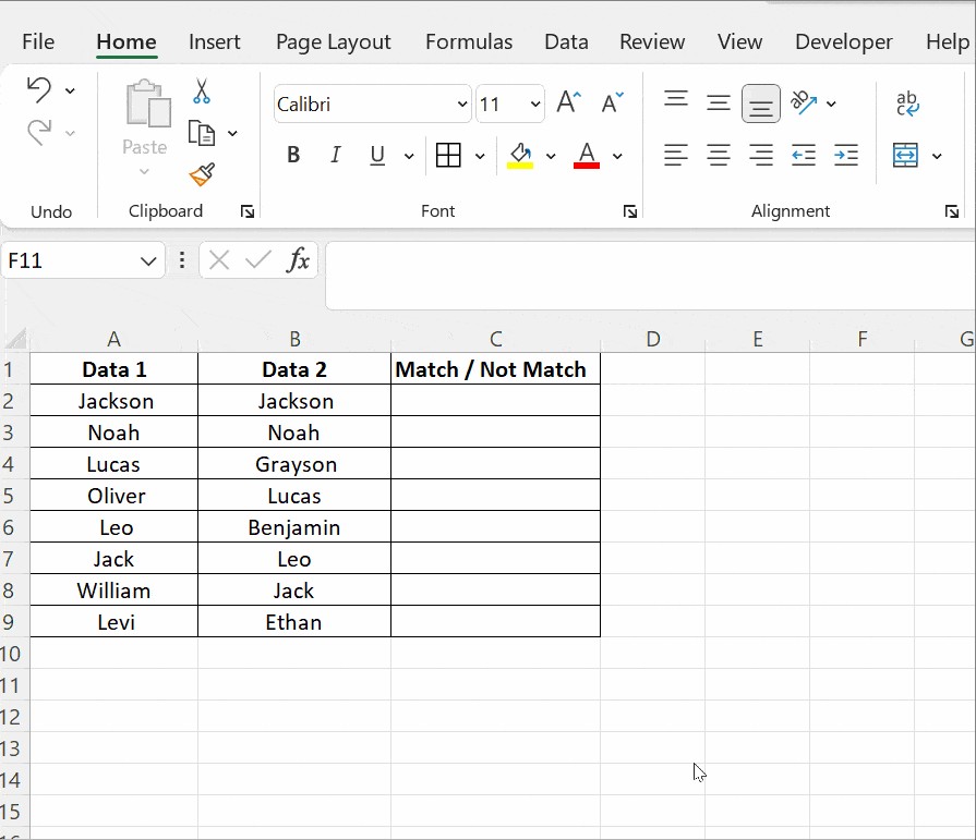
2. The IF Formula: Adding Context with “Match” and “Mismatch”
While TRUE/FALSE is informative, you might prefer more descriptive results like “Match” or “Mismatch”. The IF formula allows you to customize the output based on the comparison result, making it more user-friendly.
Formula: =IF(A2=B2,"Match","Mismatch")
Variations:
- Display “Match” or Leave Blank for Mismatches:
=IF(A2=B2,"Match","")This variation will show “Match” for identical rows and leave the cell blank if there’s a mismatch, providing a cleaner visual focus on matches. - Highlighting Differences (“Mismatch” for Differences):
=IF(A2<>B2,"Mismatch","Match")By using the “not equal to” operator (<>), you can reverse the logic to specifically highlight rows where the columns differ.
How it works:
- In an empty column (e.g., Column C), in the first row of data, enter the desired IF formula (e.g.,
=IF(A2=B2,"Match","Mismatch")). - Press Enter. Cell C2 will now display “Match” if A2 and B2 are the same, and “Mismatch” if they are different.
- Drag the fill handle down to apply the formula to the remaining rows.
Example:
| Column A (Product ID) | Column B (Product ID – Updated) | Column C (Comparison Result) |
|---|---|---|
| PID-123 | PID-123 | Match |
| PID-456 | PID-789 | Mismatch |
| PID-789 | PID-789 | Match |
| PID-001 | PID-002 | Mismatch |
The IF formula provides more context than the simple equals operator, making it easier to interpret the comparison results at a glance.
3. The EXACT Function: Case-Sensitive Comparisons
In most cases, Excel comparisons are case-insensitive, meaning “Apple” is considered the same as “apple”. However, if you need a case-sensitive comparison, the EXACT function is the solution.
Formula: =IF(EXACT(A2,B2),"Match","Mismatch")
EXACT Function Syntax: =EXACT(text1, text2)
text1: The first text string to compare.text2: The second text string to compare.
The EXACT function returns TRUE if text1 and text2 are exactly the same, including case, and FALSE otherwise.
How it works:
- In an empty column, enter the formula
=IF(EXACT(A2,B2),"Match","Mismatch"). - Press Enter and drag the fill handle down.
Example:
| Column A (Name) | Column B (Name) | Column C (Case-Sensitive Comparison) |
|---|---|---|
| John Smith | John Smith | Match |
| Apple | apple | Mismatch |
| EXCEL | Excel | Mismatch |
| Data | Data | Match |
The EXACT function is crucial when case sensitivity is important, such as when comparing product codes, usernames, or any data where capitalization matters.
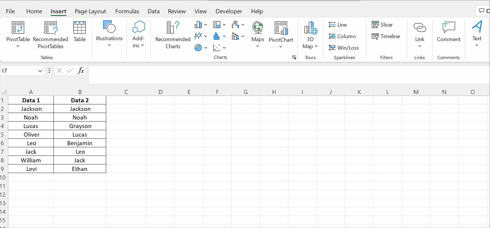
4. Conditional Formatting: Visualizing Matches and Differences
For a purely visual approach without adding extra columns for formulas, Conditional Formatting is incredibly effective. It allows you to highlight cells based on whether they are duplicates (matches) or unique (differences) across two columns.
Steps:
-
Select the columns you want to compare (e.g., Column A and Column B).
-
Go to the Home tab on the Excel ribbon.
-
Click on Conditional Formatting in the Styles group.
-
Select Highlight Cells Rules, then choose Duplicate Values…
-
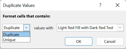
In the “Duplicate Values” dialog box:
- Choose Duplicate from the dropdown menu to highlight values that appear in both selected columns (matches).
- Choose Unique to highlight values that appear in only one of the selected columns (differences).
- Select the desired formatting style (e.g., fill color, text color, border). You can choose from preset options or select “Custom Format…” for more control.
-
Click OK.
Example using “Duplicate” to highlight matches:
By selecting “Duplicate,” Excel will highlight values that are present in both Column A and Column B with the chosen formatting. Conversely, selecting “Unique” will highlight values that are present in only one of the columns.
Conditional formatting is excellent for quickly visualizing matches and differences, especially in smaller datasets, without cluttering your spreadsheet with extra columns. You can easily clear the formatting later by going to Conditional Formatting → Clear Rules → Clear Rules from Selected Cells.
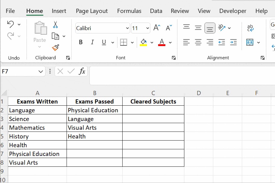
5. LOOKUP Formulas (VLOOKUP): Checking for Presence in Another Column
The VLOOKUP function is incredibly versatile for comparing columns and determining if values from one column exist in another. While primarily used for retrieving related data, it can be adapted for column comparison by simply checking if a value from one column can be found in the other.
Formula: =VLOOKUP(A2,$B$2:$B$5,1,FALSE)
VLOOKUP Function Syntax (in this context): =VLOOKUP(lookup_value, table_array, col_index_num, range_lookup)
lookup_value: The value you want to search for (e.g.,A2).table_array: The range in the second column where you want to search for thelookup_value(e.g.,$B$2:$B$5). The$symbols create absolute references, ensuring the range remains fixed when you drag the formula down.col_index_num: Always set to1in this comparison context, as we are only interested in whether the value is found, not in retrieving a value from a different column.range_lookup: Set toFALSE(or0) for an exact match. This is crucial for accurate column comparison.
How it works:
- In an empty column (e.g., Column C), enter the formula
=VLOOKUP(A2,$B$2:$B$5,1,FALSE). Adjust thetable_array($B$2:$B$5) to cover the entire range of the second column you are comparing against. - Press Enter and drag the fill handle down.
Results:
- If the value from Column A (e.g., A2) is found in Column B, VLOOKUP will return that value itself.
- If the value from Column A is not found in Column B, VLOOKUP will return the error
#N/A.
Example:
| Column A (Subjects Taken) | Column B (Subjects Passed) | Column C (VLOOKUP Result) |
|---|---|---|
| Math | Science | #N/A |
| Science | History | Science |
| English | Math | #N/A |
| History | English | History |
In this example, Column C shows the subjects from Column A that are also present in Column B. The #N/A indicates subjects taken that were not passed (not found in the “Subjects Passed” column).
You can further enhance the VLOOKUP result using the IFERROR function to replace #N/A with a more user-friendly message like “Not Found” or “Mismatch” (see “Advanced Tips” section below).
Advanced Tips and Considerations
- Comparing Columns Across Different Sheets: To compare columns located in different sheets within the same Excel workbook, simply include the sheet name in your formulas. For example, to compare Column A in “Sheet1” with Column A in “Sheet2”, in “Sheet1” you would use a formula like
=Sheet2!A2=A2. Replace “Sheet2” with the actual name of your second sheet. - Handling Errors (Using IFERROR with VLOOKUP): The
#N/Aerror from VLOOKUP can be replaced with more descriptive text using theIFERRORfunction. For example,=IFERROR(VLOOKUP(A2,$B$2:$B$5,1,FALSE), "Not Found")will display “Not Found” instead of#N/Awhen a value is not found. This makes the results more readable and easier to understand. - Performance for Large Datasets: While these formulas are efficient, comparing very large datasets (hundreds of thousands of rows) can slow down Excel. For extremely large datasets, consider using Excel’s Power Query feature or programming solutions like VBA (Visual Basic for Applications) for optimized performance. Power Query is particularly useful for data manipulation and comparison across multiple sources and large tables.
Frequently Asked Questions (FAQs)
1. What is the easiest way to compare two columns in Excel for simple matches?
The easiest methods for simple match detection are using the Equals Operator (=) for row-by-row comparison and Conditional Formatting to visually highlight duplicate values across the two columns.
2. How do I find only the differences between two columns in Excel?
To find only the differences, you can use:
- IF Formula with the “Not Equal To” operator (<>):
=IF(A2<>B2, "Different", "")will mark rows where columns differ. - Conditional Formatting with “Unique” values: Highlighting “Unique” values in Conditional Formatting will visually emphasize the entries that are different between the two selected columns.
3. Can I compare columns in Excel case-sensitively?
Yes, use the EXACT function for case-sensitive comparisons. The formula =IF(EXACT(A2,B2),"Match","Mismatch") will only register a “Match” if the text values are identical, including capitalization.
4. How can I compare two columns and return a value from another column based on the comparison?
While VLOOKUP in this context primarily checks for presence, for more complex scenarios where you need to compare columns and retrieve related data based on matches, consider using INDEX-MATCH. INDEX-MATCH is a more flexible and powerful alternative to VLOOKUP for advanced lookup and comparison tasks, especially when dealing with more complex data structures or needing to look up values in columns to the left of the lookup column.
5. Is there an Excel formula to compare two columns and highlight the differences visually?
Yes, Conditional Formatting is the best way to visually highlight differences. Use the “Unique” values rule within Conditional Formatting to automatically highlight cells that contain unique entries when comparing two columns.
Conclusion
Mastering excel formula to compare two columns is an essential skill for anyone working with data in Excel. From the simplicity of the equals operator to the power of VLOOKUP and the visual clarity of conditional formatting, Excel offers a toolkit to handle various comparison needs efficiently. By understanding and applying these techniques, you can save time, improve accuracy, and unlock valuable insights from your data. Experiment with these formulas, practice with your own datasets, and you’ll be well-equipped to tackle any column comparison task Excel throws your way, transforming raw data into actionable intelligence.