Comparing Two Columns in Excel: A Comprehensive Guide

Microsoft Excel is an indispensable tool for data management and analysis across various industries. Whether you’re managing sales figures, inventory lists, or research data, the ability to effectively compare columns is crucial for data integrity and insightful decision-making. When dealing with small datasets, manual comparison might seem feasible. However, as spreadsheets grow and data complexity increases, manual methods become time-consuming, error-prone, and simply impractical.

This guide will explore various efficient methods for Comparing Two Columns In Excel, ranging from simple formulas to more advanced features like conditional formatting and lookup functions. By mastering these techniques, you can significantly streamline your data analysis workflow, identify discrepancies, highlight matches, and extract valuable insights from your spreadsheets, regardless of their size or complexity.

We will delve into practical, step-by-step approaches, empowering you to confidently compare columns and unlock hidden patterns within your data. Let’s explore the essential techniques that will transform how you analyze and manage your data in Excel.

Why Comparing Columns in Excel is a Core Skill

Excel’s power lies in its ability to organize and manipulate data for informed decision-making. Data analysts, marketers, sales professionals, and countless others rely on Excel to extract meaningful information. In this data-driven environment, the accuracy and completeness of data are paramount.

Spreadsheets often contain interconnected data, sometimes spanning multiple sheets or even workbooks. Inconsistencies or missing data can have a ripple effect, leading to flawed analyses and misguided decisions. Comparing two columns in Excel becomes essential for data validation, identifying duplicates, spotting missing entries, and ensuring data integrity across your spreadsheets.

Imagine you are managing a product catalog and need to update pricing. You might have a master price list and a separate sheet with updated prices. Comparing these two columns allows you to quickly identify which items have price changes and ensure your system reflects the latest information. Without efficient comparison methods, this task could become a manual, lengthy, and error-prone process.

Excel provides the tools to automate and simplify this process. Whether you need to highlight matching entries, identify unique values, or perform a row-by-row comparison, understanding these methods will save you time and improve the accuracy of your data analysis. Excel can display comparison results as TRUE/FALSE, “Match”/”Not Match,” or custom messages, providing clear and immediate insights.

Methods for Comparing Two Columns in Excel

Depending on your specific needs and the type of data you are working with, Excel offers a variety of methods to compare two columns. The best approach will depend on what you want to achieve: are you looking for exact matches, unique values, differences, or simply a visual representation of the comparison?

Here are the primary methods we will explore in detail:

Using the Equals Operator (=): For basic row-by-row comparison to find exact matches.
Leveraging the IF Condition: To display custom messages like “Match” or “Not Match” based on comparison results.
Employing the EXACT() Function: For case-sensitive comparisons, ensuring text strings are identical in every aspect, including capitalization.
Conditional Formatting: To visually highlight duplicate or unique values directly within the columns, without needing extra columns.
Utilizing LOOKUP Functions (VLOOKUP): To check if values in one column exist in another column and retrieve related information, particularly useful for larger datasets.

Let’s delve into each of these methods, providing step-by-step instructions and practical examples to help you master column comparison in Excel.

1. Comparing Columns with the Equals Operator (=)

The simplest method for comparing two columns in Excel is using the equals operator (=). This performs a row-by-row comparison, checking if the values in corresponding rows of two columns are identical. The result is a logical TRUE or FALSE value, indicating whether the values match.

For example, if you have data in column A and column B, and you want to compare row 2 of both columns, you would use the formula =A2=B2.

Step-by-step guide:

Select the first cell in an empty column where you want to display the comparison results (e.g., cell C2).
Enter the formula =A2=B2 (adjust cell references as needed to match your columns).
Press Enter. The cell will display TRUE if the values in A2 and B2 are the same, and FALSE if they are different.
Drag the fill handle (the small square at the bottom-right corner of the selected cell) down to apply the formula to the rest of the rows in your data.

Column C will now show TRUE or FALSE for each row, clearly indicating whether the values in columns A and B match in that row.

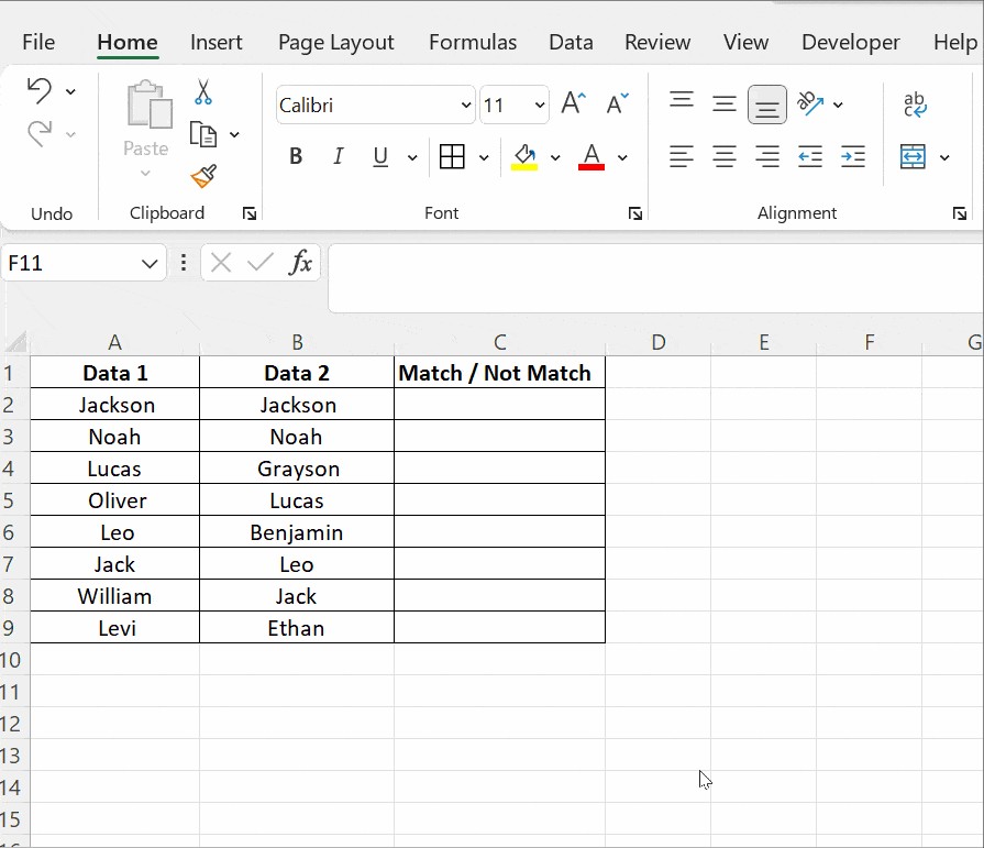
2. Comparing Columns Using the IF Condition

While the equals operator provides a basic TRUE/FALSE result, the IF condition allows for more descriptive and user-friendly outputs. You can use the IF function to display custom messages like “Match” or “Not Match” instead of TRUE/FALSE.

The basic syntax for using IF to compare two columns is: =IF(A2=B2, "Match", "Not Match").

Step-by-step guide:

Select the first cell in an empty column for results (e.g., cell C2).
Enter the formula =IF(A2=B2, "Match", "Not Match") (adjust cell references as needed).
Press Enter. The cell will now display “Match” if A2 and B2 are the same, and “Not Match” if they are different.
Drag the fill handle down to apply the formula to the remaining rows.

Finding Mismatches:

You can easily adapt the IF formula to specifically highlight mismatches. To leave the cell blank if there’s a match and display “Not Match” only for differences, use: =IF(A2=B2, "", "Not Match").

Alternatively, to explicitly show “Match” for matches and “Not a Match” for mismatches, as demonstrated in the original article, use: =IF(A2=B2, "Match", "Not a Match").

Comparing for Differences (Not Equal):

To find rows where the values in two columns are different, you can use the “not equal to” operator (<>) within the IF condition: =IF(A2<>B2, "Different", "Same"). This will return “Different” if the values in A2 and B2 are not the same, and “Same” otherwise.

3. Case-Sensitive Comparison with the EXACT() Function

The equals operator and IF condition, by default, perform case-insensitive comparisons in Excel. This means that “Apple” and “apple” would be considered a match. If you need a case-sensitive comparison, where capitalization matters, you should use the EXACT() function.

The EXACT() function compares two text strings and returns TRUE only if they are exactly the same, including case. The syntax is =EXACT(text1, text2).

Step-by-step guide for case-sensitive comparison:

Select a cell for results (e.g., C2).
Enter the formula =IF(EXACT(A2, B2), "Match", "Mismatch").
Press Enter and drag the fill handle down.

This formula first uses EXACT(A2, B2) to perform a case-sensitive comparison. If EXACT() returns TRUE (strings are identical including case), the IF function displays “Match”; otherwise, it displays “Mismatch”.

For instance, if A2 contains “Excel” and B2 contains “excel”, A2=B2 would return TRUE (case-insensitive match), but EXACT(A2, B2) would return FALSE (case-sensitive mismatch).

4. Highlighting Matches and Differences with Conditional Formatting

Conditional formatting offers a powerful visual way to compare two columns in Excel directly within the columns themselves, without needing a separate results column. You can highlight duplicate values (matches) or unique values (differences) based on your comparison.

Highlighting Duplicate Values (Matches):

Select both columns you want to compare (e.g., columns A and B).
Go to the Home tab on the Excel ribbon.
Click on Conditional Formatting in the Styles group.
Choose Highlight Cells Rules and then Duplicate Values.
In the “Duplicate Values” dialog box:
- Ensure “Duplicate” is selected in the dropdown.
- Choose a formatting style (e.g., “Light Red Fill with Dark Red Text”) from the “with” dropdown or select “Custom Format…” for more options.
Click OK.

Excel will now highlight all values that appear in both selected columns, visually representing the matches.

Highlighting Unique Values (Differences):

To highlight values that are unique to each column (i.e., values that appear in one column but not the other), follow similar steps but choose “Unique” in the “Duplicate Values” dialog box instead of “Duplicate.”

Select both columns.
Home > Conditional Formatting > Highlight Cells Rules > Duplicate Values.
In the “Duplicate Values” dialog box:
- Choose Unique from the dropdown.
- Select a formatting style.
Click OK.

Now, Excel will highlight values that are present only in one of the selected columns, visually indicating the differences.

Clearing Conditional Formatting:

To remove conditional formatting, select the formatted cells, go to Home > Conditional Formatting > Clear Rules, and choose either “Clear Rules from Selected Cells” or “Clear Rules from Entire Sheet.”

5. Using VLOOKUP for Column Comparison

The VLOOKUP function is a powerful tool for comparing two columns in Excel, especially when you need to check if values from one column exist in another and potentially retrieve related information. While primarily used for looking up values in a table, it can be effectively adapted for column comparison.

In the context of column comparison, VLOOKUP can check if a value from one column (the lookup value) exists in another column (the lookup range). If it finds a match, it can return a value from the lookup range (or #N/A if no match is found).

Example Scenario: You have a list of products in Column A (List 1) and another list of products in Column B (List 2). You want to know which products from List 1 are also present in List 2.

Step-by-step guide using VLOOKUP:

Select a cell in an empty column next to List 1 (e.g., C2).
Enter the formula =VLOOKUP(A2, $B$2:$B$5, 1, FALSE) (adjust the range $B$2:$B$5 to cover the entire List 2).
- A2: The lookup value (the first product in List 1).
- $B$2:$B$5: The lookup range (List 2, using absolute references $).
- 1: The column index (we want to return a value from the first column of the lookup range, which is List 2 itself).
- FALSE: Specifies an exact match (we want to find exact product names).
Press Enter and drag the fill handle down.

Interpreting VLOOKUP Results:

If VLOOKUP finds a match, it will return the matching value from List 2 (in this case, the product name itself).
If VLOOKUP does not find a match for a product from List 1 in List 2, it will return #N/A.

You can then easily filter or sort column C to identify the #N/A values, which represent the products in List 1 that are not found in List 2.

Combining VLOOKUP with IF for Custom Messages:

To display more user-friendly messages, you can combine VLOOKUP with the IFERROR function or the IF function along with ISNA() to handle the #N/A errors.

Using IFERROR: =IFERROR(VLOOKUP(A2, $B$2:$B$5, 1, FALSE), "Not Found"). This will display “Not Found” if VLOOKUP returns #N/A, and the matching value otherwise.
Using IF and ISNA: =IF(ISNA(VLOOKUP(A2, $B$2:$B$5, 1, FALSE)), "Not Found", "Found"). This will display “Not Found” if VLOOKUP returns #N/A (ISNA returns TRUE for #N/A), and “Found” if a match is found.

Frequently Asked Questions about Comparing Columns in Excel

1. What is a quick way to visually compare two columns for differences without formulas?

Excel’s “Go To Special” feature offers a fast way to highlight row differences between two columns. Select both columns, go to Home → Find & Select → Go To Special, choose Row Differences, and click OK. Cells with matching data across rows will appear white, while unmatched cells will be highlighted (usually in gray).

2. How can I compare more than two columns in Excel using IF conditions?

For tables with three or more columns, you can use nested IF statements or combine IF with logical functions like AND or OR.

To find rows where all cells in multiple columns match: Use AND within the IF formula. For example, =IF(AND(A2=B2, A2=C2), "Full Match", "") checks if A2, B2, and C2 are all equal.
To find rows where at least two cells in multiple columns match: Use OR within the IF formula. For example, =IF(OR(A2=B2, B2=C2, A2=C2), "Match", "") checks if any two cells among A2, B2, and C2 are equal.

3. Can I use INDEX-MATCH instead of VLOOKUP for column comparison?

Yes, INDEX-MATCH is a more flexible and often preferred alternative to VLOOKUP. For column comparison, you would primarily use the MATCH function to find matches and handle #N/A errors similarly to VLOOKUP.

For example, to check if values in column D exist in column A and return a corresponding value from column B, you could use: =IFERROR(INDEX($B$2:$B$4, MATCH(D2, $A$2:$A$4, 0)), "#N/A"). This formula uses MATCH to find the position of D2 within the range A2:A4 and then INDEX to retrieve the value from column B at that position. IFERROR handles cases where no match is found.

Conclusion: Mastering Column Comparison in Excel

Effectively comparing two columns in Excel is a fundamental skill for anyone working with data. This guide has provided a comprehensive overview of various methods, from basic operators and IF conditions to conditional formatting and powerful lookup functions like VLOOKUP.

By understanding and applying these techniques, you can significantly enhance your data analysis capabilities, improve data accuracy, and save valuable time when working with spreadsheets of any size. Experiment with these methods, adapt them to your specific needs, and unlock the full potential of Excel for data comparison and analysis.

To further expand your Excel skills, consider exploring advanced lookup functions like XLOOKUP and delving deeper into conditional formatting options. Continued learning and practice will solidify your expertise and make you a more proficient Excel user.